Python demo — a script that recomputes what this entry states and prints one line per check
A kernel method applies a linear method, such as a
linear model or a linear classifier, to transformed
feature vectors.
The transformation is constructed from a kernel:
each feature vector is mapped to a function
with domain equal to the original feature space, and
inner products between transformed feature vectors reduce to
evaluations of a kernel. Kernel methods offer great
flexibility in the choice of the feature space, which can
consist of text documents or discrete structures such as
graphs.
Definition
A kernel method is a machine learning (ML) method that
applies a linear method, such as a linear model for regression or
a linear classifier for classification, to transformed
feature vectors that are constructed from a kernel
(Lampert, 2009; Schölkopf and Smola, 2002). Kernel
methods are used in computer vision to decide whether an image shows
a specific object (Lampert, 2009), and in natural language processing (NLP) to
classify text documents by topic
(Cristianini and Shawe-Taylor, 2000).
Linear methods learn a hypothesis that combines the
features of a data point linearly, e.g.,
$\hypothesis(\featurevec) = \weights^{\top} \featurevec$ for the
feature space $\featurespace = \reals^{\nrfeatures}$. Such a
hypothesis predicts well only if the relation between the
feature vectors and the labels of data points is
approximately linear. Moreover, a linear
method requires numeric feature vectors and is not directly
applicable to data points from an arbitrary feature space
$\featurespace$, such as text documents or graphs.
B-linearBoth limitations can be mitigated by a feature transformation
$\featuretrafo: \featurespace \rightarrow \hilbertspace$ from the original
feature space $\featurespace$ to a transformed feature space
$\hilbertspace$, chosen as a Hilbert space.
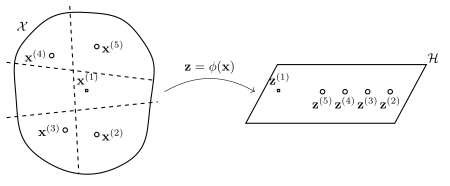
Fig. 1 shows a binary classification problem
with the first limitation: no straight line separates the two
classes in the original feature space. A suitable
feature transformation makes a dataset "more linear": the relation
between the transformed feature vectors $\featuretrafo(\featurevec)$
and the labels is closer to linear in $\hilbertspace$ than the
relation between the original feature vectors $\featurevec$ and
the labels is in $\featurespace$.
Figure 1: Five data points characterized by feature vectors $\featurevec^{(\sampleidx)}$
and labels $\truelabel^{(\sampleidx)} \in \{ \circ, \square \}$ for $\sampleidx=1, \,\ldots, \,5$.
The curved boundary indicates the original feature space $\featurespace$ (left);
the parallelogram indicates a section of the transformed feature space
$\hilbertspace$ (right), which is a linear space (see Hilbert space).
With these feature vectors, there is no way to separate the two classes
by a straight line (representing the decision boundary of a linear classifier).
The dashed lines illustrate three failed attempts: each places the
feature vector $\featurevec^{(1)}$ (class $\square$) on the same side
as at least one feature vector of class $\circ$, so a linear classifier
with any of these decision boundaries misclassifies at least
one data point.
In contrast, the transformed feature vectors $\vz^{(\sampleidx)} = \featuretrafo\big(\featurevec^{(\sampleidx)}\big)$
allow the data points to be separated using a linear classifier
A useful feature transformation $\featuretrafo$ often delivers transformed
feature vectors in a Hilbert space $\hilbertspace$ of high
(possibly infinite) dimension (Schölkopf and Smola, 2002). Computing and
storing the transformed feature vectors $\featuretrafo(\featurevec)$
explicitly can then be infeasible. However, linear methods access the
feature vectors of data points only through
inner products between pairs of feature vectors (see
linear model). For example, the prediction delivered by a
trained support vector machine (SVM) is a weighted sum of inner products between the
feature vector of a new data point and the feature vectors in
the training set. To apply a linear method to the transformed
feature vectors, it is therefore enough to know the
inner products
$\innerprod{\featuretrafo(\featurevec)}{\featuretrafo(\featurevec')}$ for
every possible pair of feature vectors
$\featurevec, \featurevec' \in \featurespace$. These
inner products are captured by a single function of two
arguments, the kernel defined by
\[
\kernelmap{\featurevec}{\featurevec'}
\defeq \innerprod{\featuretrafo(\featurevec)}{\featuretrafo(\featurevec')}
\text{, for } \featurevec, \featurevec' \in \featurespace \text{.}
\]
The value $\kernelmap{\featurevec}{\featurevec'}$ quantifies the
similarity of the feature vectors $\featurevec$ and $\featurevec'$.
As an inner product of transformed feature vectors, the
kernel is symmetric, and every matrix of pairwise
kernel values is positive semi-definite (psd); these two properties characterize
kernels.
A linear method that is applied to the transformed feature vectors
thus requires only the kernel $\kernel$; the feature transformation
$\featuretrafo$ itself is never evaluated.
Kernel methods reverse this construction: they start from a
kernel $\kernel: \featurespace \times \featurespace \rightarrow \reals$
and construct the feature transformation from it. The
feature transformation sends a feature vector $\featurevec \in \featurespace$
to the function $\kernelmap{\featurevec}{\cdot}$, i.e., the
transformed feature vector
$\vz \defeq \featuretrafo(\featurevec) = \kernelmap{\featurevec}{\cdot}$
is itself a function with domain $\featurespace$, for every
$\featurevec \in \featurespace$. These
functions belong to the reproducing kernel Hilbert space (RKHS) $\hilbertspace_{\kernel}$
associated with the kernel $\kernel$ (Aronszajn, 1950). The
inner product between the transformed feature vectors of two
original feature vectors $\featurevec, \featurevec' \in \featurespace$
is a single kernel evaluation,
\[
\innerprod{\kernelmap{\featurevec}{\cdot}}{\kernelmap{\featurevec'}{\cdot}}
= \kernelmap{\featurevec}{\featurevec'} \text{.}
\]
More generally, the inner product between the transformed
feature vector $\kernelmap{\featurevec}{\cdot}$ and any function
$\hypothesis \in \hilbertspace_{\kernel}$ is a point evaluation,
\[
\innerprod{\hypothesis}{\kernelmap{\featurevec}{\cdot}} = \hypothesis(\featurevec) \text{,}
\]
which is referred to as the reproducing property of the RKHS
$\hilbertspace_{\kernel}$ (Aronszajn, 1950). This reproducing property
contains
$\innerprod{\kernelmap{\featurevec}{\cdot}}{\kernelmap{\featurevec'}{\cdot}}
= \kernelmap{\featurevec}{\featurevec'}$ as a special case which is
obtained for the choice $\hypothesis = \kernelmap{\featurevec'}{\cdot}$.
The (possibly infinite-dimensional) transformed feature vectors
therefore never need to be computed explicitly.
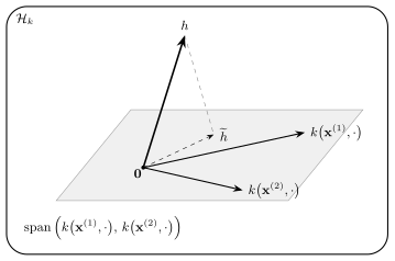
Fig. 2 depicts the RKHS
$\hilbertspace_{\kernel}$ for a training set with two
data points: a hypothesis $\hypothesis$ is a single
vector in $\hilbertspace_{\kernel}$. The value
$\innerprod{\hypothesis}{\kernelmap{\featurevec}{\cdot}} = \hypothesis(\featurevec)$
is a linear function of the transformed feature vector
$\kernelmap{\featurevec}{\cdot} \in \hilbertspace_{\kernel}$, but the
function $\featurevec \mapsto \hypothesis(\featurevec)$ induced
on the original feature space $\featurespace$ is nonlinear in
general. Linearity in the original feature vector $\featurevec$ may
not even be defined, since the feature space $\featurespace$ need
not be a vector space, e.g., when it consists of text documents
or graphs.
Figure 2: The RKHS $\hilbertspace_{\kernel}$ for a training set
with two data points having feature vectors
$\featurevec^{(1)}, \featurevec^{(2)}$. Their transformed
feature vectors $\kernelmap{\featurevec^{(1)}}{\cdot}$ and
$\kernelmap{\featurevec^{(2)}}{\cdot}$ span a two-dimensional
subspace (shaded parallelogram). A hypothesis $\hypothesis$ is a
vector in $\hilbertspace_{\kernel}$; its prediction
for a data point with feature vector $\featurevec$ is the
inner product $\innerprod{\hypothesis}{\kernelmap{\featurevec}{\cdot}} = \hypothesis(\featurevec)$.
This prediction is a linear function of the
transformed feature vector $\kernelmap{\featurevec}{\cdot}$,
but the function $\featurevec \mapsto \hypothesis(\featurevec)$
induced on $\featurespace$ is nonlinear in general.
Replacing $\hypothesis$ by its orthogonal projection
$\widetilde{\hypothesis}$ (dashed arrow) onto the shaded subspace
leaves the predictions for both data points in the
training set unchanged and never increases
$\normgeneric{\hypothesis}{\hilbertspace_{\kernel}}$
Kernel methods can be formulated as regularized empirical risk minimization (RERM) over the RKHS
$\hilbertspace_{\kernel}$,
\[
\min_{\hypothesis \in \hilbertspace_{\kernel}} \frac{1}{\samplesize}
\sum_{\sampleidx=1}^{\samplesize}
\lossfunc{\big(\featurevec^{(\sampleidx)}, \truelabel^{(\sampleidx)}\big)}{\hypothesis}
+ \regparam \normgeneric{\hypothesis}{\hilbertspace_{\kernel}}^{2}
\text{,}
\]
over a training set with feature vectors $\featurevec^{(\sampleidx)}$
and labels $\truelabel^{(\sampleidx)}$, for
$\sampleidx = 1, \ldots, \samplesize$, and with a
regularization parameter $\regparam > 0$ that weights the
penalty term $\normgeneric{\hypothesis}{\hilbertspace_{\kernel}}^{2}$. The loss function
$\lossfunc{\big(\featurevec^{(\sampleidx)}, \truelabel^{(\sampleidx)}\big)}{\hypothesis}$
depends on $\hypothesis$ only through the prediction
$\hypothesis\big(\featurevec^{(\sampleidx)}\big)$, i.e., it is a function
of the prediction $\hypothesis\big(\featurevec^{(\sampleidx)}\big)$ and the
label $\truelabel^{(\sampleidx)}$ only. Since
$\hypothesis \in \hilbertspace_{\kernel}$, the reproducing property
delivers this prediction as an inner product,
$\hypothesis\big(\featurevec^{(\sampleidx)}\big) = \innerprod{\hypothesis}{\kernelmap{\featurevec^{(\sampleidx)}}{\cdot}}$.
By the representer theorem, this optimization problem has a minimizer
of the form $\widehat{\hypothesis} = \sum_{\sampleidx=1}^{\samplesize} \expcoeff_{\sampleidx} \kernelmap{\featurevec^{(\sampleidx)}}{\cdot}$
with expansion coefficients
$\expcoeff_{1}, \ldots, \expcoeff_{\samplesize} \in \reals$
(Schölkopf and Smola, 2002). Fig. 2
illustrates the underlying projection argument: replacing a
hypothesis $\hypothesis$ by its orthogonal projection
$\widetilde{\hypothesis}$ onto the subspace spanned by
$\kernelmap{\featurevec^{(1)}}{\cdot}, \ldots, \kernelmap{\featurevec^{(\samplesize)}}{\cdot}$
leaves the predictions on the training set unchanged and
never increases the penalty term; hence some minimizer
$\widehat{\hypothesis}$ lies in this subspace and has the above
form.
B-kernelTraining thus reduces to a
convex optimization problem in these $\samplesize$ coefficients, and
the prediction $\widehat{\hypothesis}(\featurevec) = \sum_{\sampleidx=1}^{\samplesize} \expcoeff_{\sampleidx} \kernelmap{\featurevec^{(\sampleidx)}}{\featurevec}$
requires only kernel evaluations. Examples of such kernel
methods are the kernel SVM, obtained for the
hinge loss, and kernel ridge regression, obtained for the
squared error loss
(Cristianini and Shawe-Taylor, 2000; Hastie et al., 2009, Ch. 12).
For $\featurespace = \reals^{\nrfeatures}$, a widely used choice of
the kernel $\kernel$ is the Gaussian kernel
$\kernelmap{\featurevec}{\featurevec'} = \exp\big(- \normgeneric{\featurevec - \featurevec'}{2}^{2} / (2 \sigma^{2}) \big)$
with bandwidth $\sigma > 0$. Kernels are also available for
data points without numeric features, such as strings and
graphs (Schölkopf and Smola, 2002).
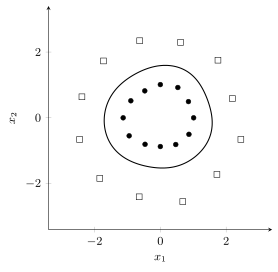
Fig. 3 shows the nonlinear
decision boundary $\widehat{\hypothesis}(\featurevec) = 0$ of a
hypothesis $\widehat{\hypothesis}$ learned by a
Gaussian-kernel method with squared error loss
from a training set of two concentric rings that no
linear classifier separates. Here kernel ridge regression fits the
labels $\truelabel^{(\sampleidx)} \in \{-1, +1\}$ and the
prediction is the sign of the fitted value, a construction
referred to as regularized least-squares classification
(Rifkin et al., 2003).
Figure 3: A Gaussian-kernel method (kernel ridge regression
with $\sigma = 0.8$,
$\regparam = 10^{-3}$) trained on a training set of two
concentric rings. Data points with label
$\truelabel = +1$ are drawn as filled circles, those with
$\truelabel = -1$ as open squares. The decision boundary
$\widehat{\hypothesis}(\featurevec) = 0$ of the learned
hypothesis (solid closed curve) encircles the
inner ring. Note that the dataset is not linearly separable
in the original feature space. Data generated by
pythondemos/kernelmethod.py
Kernel methods impose the smoothness assumption through the
RKHS norm. That norm
$\normgeneric{\hypothesis}{\hilbertspace_{\kernel}}$ quantifies the smoothness of
a hypothesis $\hypothesis$: it is large for a rapidly varying
$\hypothesis$ and small for a smooth $\hypothesis$. Moreover,
different kernels impose different kinds of smoothness.
The Gaussian kernel gives infinitely differentiable
functions and penalizes high-frequency components. The
Mat\'ern kernels are a family of kernels indexed by a
smoothness parameter $\nu > 0$: their RKHS coincides,
with equivalent norms, with the Sobolev space of order
determined by $\nu$, whose functions have derivatives
up to that order in the weak sense
(Rasmussen and Williams, 2006, Eq. 4.15;
Kanagawa et al., 2018, Example 2.6). Because the penalty term
$\regparam \normgeneric{\hypothesis}{\hilbertspace_{\kernel}}^{2}$
in the above RERM is the squared RKHS norm,
it implements smoothness as quantified by
$\normgeneric{\hypothesis}{\hilbertspace_{\kernel}}$: among
hypotheses with the same training error, the
RERM objective function is smallest for the hypothesis
with the smallest RKHS norm.
The choice of kernel shapes not only training
but also the predictions of the learned hypothesis:
for localized kernels, such as the Gaussian kernel, the
prediction $\widehat{\hypothesis}(\featurevec)$ is dominated
by the data points in the training set whose
feature vectors are close to $\featurevec$. In this sense, kernel
methods implement the smoothness assumption: data points
with nearby feature vectors obtain similar predictions. The
locality of the predictions also makes kernel methods a
soft-weighted analogue of $k$-nearest neighbors ($k$-NN): instead of averaging the
labels of a fixed number of nearest data points, the
prediction weights all data points in the training set
by the kernel value
$\kernelmap{\featurevec^{(\sampleidx)}}{\featurevec}$
(Hastie et al., 2009, Ch. 6).
Synonyms: kernel machine.
See also: kernel, feature transformation, Hilbert space,
reproducing kernel Hilbert space, linear model, linear classifier, support vector machine,
kernel ridge regression, ridge regression,
smoothness assumption, $k$-nearest neighbors.
Schölkopf and Smola (2002). Learning with Kernels: Support Vector Machines, Regularization, Optimization, and Beyond. MIT Press. doi.org/10.7551/mitpress/4175.001.0001
Cristianini and Shawe-Taylor (2000). An Introduction to Support Vector Machines and Other Kernel-based Learning Methods. Cambridge Univ. Press. doi.org/10.1017/cbo9780511801389
Hastie et al. (2009). The Elements of Statistical Learning: Data Mining, Inference, and Prediction. Springer Science+Business Media. doi.org/10.1007/978-0-387-84858-7
Rifkin et al. (2003). Regularized Least-Squares Classification. Advances in Learning Theory: Methods, Model and Applications. doi.org/10.21236/ada454981