Hilbert space

Typeset PDF version — the authoritative form of this entry

Python demo — a script that recomputes what this entry states and prints one line per check

A Hilbert space is an inner product space that is complete: every Cauchy sequence of its elements has a limit that again belongs to the space. Three examples are used throughout machine learning (ML): the Euclidean space of a fixed dimension, the space of random variables (RVs) with finite variance on a common probability space, and a reproducing kernel Hilbert space (RKHS). Linear regression uses a Euclidean space as its feature space and to parameterize its hypothesis space. Optimal estimation amounts to a projection in a Hilbert space consisting of RVs. A kernel method uses an RKHS as its transformed feature space and as its hypothesis space.

Definition

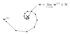
B-cauchyConsider some machine learning (ML) method with a hypothesis space that is equipped with a metric, i.e., a metric space. An iterative training method improves a hypothesis step by step, producing a sequence $\hypothesis^{(1)}, \hypothesis^{(2)}, \ldots$ of hypotheses. To ensure that this sequence converges to some optimal hypothesis $\hypothesis^{\star}$, it is necessary that the hypotheses are increasingly close to each other, i.e., that they form a Cauchy sequence. Being a Cauchy sequence is not sufficient on its own. What turns it into convergence for every such sequence is a property of the underlying metric space, namely that it is complete. A prime example of a complete metric space is a Euclidean space $\reals^{\nrfeatures}$ of finite dimension $\nrfeatures$.

B-rvspaceA Hilbert space is a generalization of a Euclidean space to possibly infinite dimensions. In particular, a Hilbert space $(\hilbertspace, \innerprod{\cdot}{\cdot})$ is an inner product space in which every Cauchy sequence of its elements has a limit that again belongs to $\hilbertspace$ (Bauschke and Combettes, 2011, Sect. 1.12) (see Fig. 1).

Figure 1 of the entry hilbertspace — Figure 1: Completeness. The elements $\vw^{(1)}, \vw^{(2)}, \ldots$ of a Cauchy sequence (dots) lie ever closer to each other, and their limit $\vw = \lim_{\sampleidx \rightarrow \infty} \vw^{(\sampleidx)}$ (cross) again belongs to the Hilbert space. Data generated by `pythondemos/hilbertspace.py`

The elements of $\hilbertspace$ are called vectors, whether they are arrays of numbers, random variables (RVs), or functions: what makes them vectors is that they can be added and scaled (see vector space). The inner product induces a norm $\normgeneric{\vu}{\hilbertspace} \defeq \sqrt{\innerprod{\vu}{\vu}}$ and, in turn, a metric $\metric{\vu}{\vv} \defeq \normgeneric{\vu - \vv}{\hilbertspace}$ (see inner product). A sequence $\vu^{(1)}, \vu^{(2)}, \ldots$ of vectors of $\hilbertspace$ is a Cauchy sequence if its vectors eventually lie within any prescribed distance of each other: for every distance $\epsilon > 0$, however small, there is an index $N$ such that $\normgeneric{\vu^{(\sampleidx)} - \vu^{(\sampleidx')}}{\hilbertspace} < \epsilon$ for all $\sampleidx, \sampleidx' \geq N$ (Rudin, 1976, Definition 3.8).

Three examples of Hilbert spaces are used throughout ML: the Euclidean space $\reals^{\featuredim}$ of feature vectors, the space of RVs with finite variance on a common probability space, and a reproducing kernel Hilbert space (RKHS) of functions. The first of them carries the standard inner product $\innerprod{\vu}{\vv} = \vu^{\top} \vv$, and its completeness follows from that of the real numbers (Rudin, 1976, Thm. 3.11). Linear regression uses the Euclidean space $\reals^{\featuredim}$ in two roles. The feature vectors $\featurevec \in \reals^{\featuredim}$ of the data points it is applied to are vectors of this space, and so are the weights $\weights \in \reals^{\featuredim}$ that parameterize its hypothesis space $\big\{ \hypothesis(\featurevec) = \innerprod{\weights}{\featurevec} \, : \, \weights \in \reals^{\featuredim} \big\}$. Gradient descent (GD) searching for those weights produces a sequence $\weights^{(1)}, \weights^{(2)}, \ldots$ of model parameters. These are vectors in the second role, so the question the opening paragraph asks has a reassuring answer here: $\reals^{\featuredim}$ is complete, and a Cauchy sequence of model parameters converges to model parameters.

The second example is the set of all RVs $x$ with finite variance, defined on a common probability space (Gray and Davisson, 2004, Sect. 5.8.1). Here, two RVs are identified whenever the expectation of their squared difference is zero, $\expect\big\{ (x - x')^{2} \big\} = 0$, i.e., whenever $x = x'$ with probability one. With this identification, the expectation $\innerprod{x}{x'} \defeq \expect\{ x x' \}$ is an inner product, and the resulting space is complete (Gray and Davisson, 2004, Lem. 5.1).

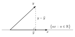
B-projIn the Hilbert space of finite-variance RVs on a common probability space, optimal linear estimation is an orthogonal projection (see Fig. 2). A linear estimator $\predictedlabel$ of an RV $\truelabel$ from an observed RV $\feature$ is an element of the subspace $\big\{ a \feature \, : \, a \in \reals \big\}$ spanned by $\feature$. The corresponding estimation error $\truelabel - \predictedlabel$ is measured by the induced norm $\sqrt{\innerprod{\truelabel - \predictedlabel}{\truelabel - \predictedlabel}}$. The smallest error is obtained by the linear estimator whose error is orthogonal to $\feature$ (Gray and Davisson, 2004, Thm. 4.9), \begin{align} 0 & = \innerprod{\truelabel - \predictedlabel}{\feature} \nonumber \\ & = \expect \big\{ \big(\truelabel - \predictedlabel \big) \feature \big\} \text{.} \nonumber \end{align} When the RVs $\truelabel,\feature$ are zero-mean, this orthogonality means that the error $\truelabel - \predictedlabel$ is uncorrelated with $\feature$.

Figure 2 of the entry hilbertspace — Figure 2: Optimal linear estimation as an orthogonal projection. The RV $\truelabel$, the observed RV $\feature$, and the estimator $\predictedlabel$ are vectors of the Hilbert space of finite-variance RVs. The estimators that are linear in $\feature$ form the subspace $\{ a \feature : a \in \reals \}$ spanned by $\feature$ (the straight line through it), and the estimation error $\truelabel - \predictedlabel$ is smallest for the $\predictedlabel$ whose error is orthogonal to $\feature$, the right angle marked by the small square at $\predictedlabel$

Optimal nonlinear estimation can also be represented as an orthogonal projection, but on a larger subspace. Projecting $\truelabel$ onto the RVs that are functions of $\feature$, rather than onto the multiples $a \feature$ alone, gives the conditional expectation $\expect\{ \truelabel \mid \feature \}$: it has the smallest squared error among all estimators computed from $\feature$ (Gray and Davisson, 2004, Thm. 4.5).

B-rkhsThe third example is an RKHS. It is a Hilbert space $\hilbertspace$ of functions $\hypothesis: \featurespace \to \reals$ whose inner product reproduces point evaluations. In particular, each RKHS is associated with a kernel $\kernelmap{\cdot}{\cdot}$ such that $\kernelmap{\featurevec}{\cdot} \in \hilbertspace$ for every $\featurevec \in \featurespace$ and \[ \hypothesis(\featurevec) = \innerprod{\hypothesis}{\kernelmap{\featurevec}{\cdot}} \quad \text{for every } \hypothesis \in \hilbertspace \text{.} \] Thus, each vector $\hypothesis \in \hilbertspace$ is itself a hypothesis map $\featurespace \to \reals$, evaluated by taking an inner product with $\kernelmap{\featurevec}{\cdot}$. This construction of a hypothesis map generalizes the linear model, which uses the standard inner product of the Euclidean space. The map $\featurevec \mapsto \kernelmap{\featurevec}{\cdot}$ is a feature transformation, carrying the feature vector of a data point into $\hilbertspace$. A kernel method uses an RKHS in two roles. It is the transformed feature space, in which a data point is represented by $\kernelmap{\featurevec}{\cdot}$, and it is the hypothesis space from which a hypothesis is learned (Hastie et al., 2009, Sect. 12.3.3; Schölkopf and Smola, 2002). These are the two roles of $\reals^{\featuredim}$ in linear regression, with one difference: there a vector parameterizes a hypothesis, here a vector is one.

See also: inner product, vector space, norm, Cauchy sequence, Euclidean space, random variable, variance, expectation, conditional expectation, reproducing kernel Hilbert space, kernel method, orthogonal projection.

References

Bauschke and Combettes (2011). Convex Analysis and Monotone Operator Theory in Hilbert Spaces. Springer Science+Business Media. doi.org/10.1007/978-1-4419-9467-7
Rudin (1976). Principles of Mathematical Analysis. mcgraw.
Gray and Davisson (2004). An Introduction to Statistical Signal Processing. Cambridge Univ. Press. ee.stanford.edu/~gray/sp.pdf
Hastie et al. (2009). The Elements of Statistical Learning: Data Mining, Inference, and Prediction. Springer Science+Business Media. doi.org/10.1007/978-0-387-84858-7
Schölkopf and Smola (2002). Learning with Kernels: Support Vector Machines, Regularization, Optimization, and Beyond. MIT Press. doi.org/10.7551/mitpress/4175.001.0001

Cite this entry

@misc{dictml_hilbertspace,
  author = {Jung, Alexander},
  title = {Hilbert space},
  howpublished = {Dictionary of Applied Machine Learning (course edition)},
  year = {2026},
  doi = {10.5281/zenodo.21569296},
  note = {ISBN 978-952-64-3013-3, CC BY 4.0, retrieved 2026-08-21},
  url = {https://dictionaryofml.org/terms/hilbertspace.html}
}