Dictionary of Applied Machine Learning
Typeset PDF version — the authoritative form of this entry
Python demo — a script that recomputes what this entry states and prints one line per check
Many machine learning (ML) applications involve data points whose features form numeric arrays. Examples include the color intensities of image pixels, the amplitudes at regular intervals of a sensor signal, and the embeddings of tokens used by large language models (LLMs). These numeric arrays can be naturally represented by vectors in some vector space. Many ML methods rely on measuring the similarity between vectors that represent data points. Each neuron of an artificial neural network (ANN) matches its input, for example the color intensities of an image, against a learned template. The attention unit of an LLM compares the query vector of a token with the key vector of another token, both formed from the embeddings of those tokens. Both comparisons compute an inner product: a number assigned to a pair of vectors in a vector space that measures their similarity.
P-arrayData points are often characterized by features that form a numeric array: the color intensities of the pixels of an image, the amplitudes of a sensor signal at regular intervals, or the embedding of a token in a large language model (LLM). Such an array can be represented by a vector, i.e., an element of a vector space. Many machine learning (ML) methods compare two data points by measuring how similar the vectors that represent them are. One principled measure of this similarity is an inner product.
P-axiomsConsider a vector space $\vecspace$ over the field of real numbers $\reals$. An inner product in $\vecspace$ is a function \[ \innerprod{\cdot}{\cdot}: \vecspace \times \vecspace \to \reals \] that satisfies the following properties for all vectors $\vu, \vv, \vw \in \vecspace$ and all scalars $\expcoeff \in \reals$ (Axler, 2024, Def. 6.2):
P-normThe pair $(\vecspace, \innerprod{\cdot}{\cdot})$ is called an inner product space. Each inner product induces a norm via $\norm{\vu} \defeq \sqrt{\innerprod{\vu}{\vu}}$ for all $\vu \in \vecspace$, which in turn induces a metric via $\metric{\vu}{\vv} \defeq \norm{\vu - \vv}$ for all $\vu, \vv \in \vecspace$.
P-cosFor the Euclidean space $\vecspace = \reals^{\featuredim}$,
the standard inner product, also called the dot product, is
$\innerprod{\featurevec}{\featurevec'} = \featurevec^{\top}
\featurevec' = \sum_{\featureidx=1}^{\featuredim} \feature_{\featureidx} \feature'_{\featureidx}$ (Strang, 2016, Sect. 1.2).
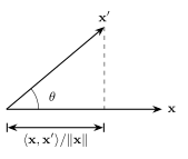
Geometrically, the inner product determines orthogonal projections:
the orthogonal projection of $\featurevec'$ onto the direction of a
nonzero vector $\featurevec$ has the signed length
$\innerprod{\featurevec}{\featurevec'} / \norm{\featurevec}$
(Axler, 2024, Example 6.56) (see Fig. 1).
For two vectors, the sign and magnitude of their inner product can be read off the angle between these vectors. The inner product is positive for $\theta < \pi/2$, zero for $\theta = \pi/2$, where the two vectors are orthogonal, and negative for $\theta > \pi/2$; and $\cos \theta$ is the inner product divided by the two norms, so it grades alignment on $[-1,1]$ without regard to length. The angle drawn in Fig. 1 is smaller than $\pi/2$: the two vectors have a positive inner product, and the orthogonal projection therefore falls on the same side of the origin as $\featurevec$.
P-projectFig. 1 projects one vector onto the direction of another, that is, onto the line it spans. The same characterization holds for a whole subspace, and it is what turns approximation problems, with respect to the induced norm, into systems of linear equations. Consider a subspace $\mathcal{U} \subseteq \vecspace$ and a vector $\vv \in \vecspace$. In general, the vector of $\mathcal{U}$ closest to $\vv$ with respect to some norm is called the projection of $\vv$ onto $\mathcal{U}$. If the norm is induced by some inner product, the projection becomes an orthogonal projection: a vector $\widehat{\vv} \in \mathcal{U}$ minimizes $\norm{\vv - \vu}$ over all $\vu \in \mathcal{U}$ if and only if the approximation error $\vv - \widehat{\vv}$ is orthogonal to every vector in $\mathcal{U}$, \begin{equation} \label{equ_orthogonality_innerproduct_dict} \innerprod{\vv - \widehat{\vv}}{\vu} = 0 \quad \text{for all } \vu \in \mathcal{U} \text{.} \end{equation} The reason is the Pythagorean identity \[ \norm{\vv - \vu}^{2} = \norm{\vv - \widehat{\vv}}^{2} + \norm{\widehat{\vv} - \vu}^{2} \text{,} \] which holds for every $\vu \in \mathcal{U}$ whenever \(\eqref{equ_orthogonality_innerproduct_dict}\) does. The second term is non-negative, so no vector of $\mathcal{U}$ is closer to $\vv$ than $\widehat{\vv}$ is: orthogonality of the error and being closest are the same condition (Axler, 2024, Thm. 6.61). The orthogonality condition \(\eqref{equ_orthogonality_innerproduct_dict}\) is linear in $\widehat{\vv}$, so a minimizer can be computed by solving linear equations.
P-convexThe characterization extends beyond subspaces. For a non-empty closed convex set $\mathcal{C} \subseteq \reals^{\featuredim}$, a vector $\widehat{\vv} \in \mathcal{C}$ is the projection of $\vv$ onto $\mathcal{C}$ if and only if \begin{equation} \label{equ_variational_inequality_dict} \innerprod{\vv - \widehat{\vv}}{\vu - \widehat{\vv}} \leq 0 \quad \text{for all } \vu \in \mathcal{C} \text{.} \end{equation} Such a projection exists and is unique (Bertsekas, 2009, Prop. 1.1.9).
P-linregOne application of the subspace case \(\eqref{equ_orthogonality_innerproduct_dict}\) is a characterization of linear regression: the learned model parameters are those for which the prediction error is orthogonal to every column of the feature matrix (see normal equations), so the resulting predictions are the orthogonal projection of the label vector onto the column space of the feature matrix. The convex case \(\eqref{equ_variational_inequality_dict}\) becomes relevant when linear regression is modified by adding a convex constraint on the model parameters.
P-weightThe Euclidean space $\reals^{\featuredim}$ carries other inner products besides the standard one (Axler, 2024, Example 6.3). As a case in point, each symmetric and positive definite (pd) matrix $\mA \in \reals^{\featuredim \times \featuredim}$ induces an inner product $\innerprod{\featurevec}{\featurevec'} \defeq \featurevec^{\top} \mA \featurevec'$. Such a matrix weighs the coordinate directions against each other, and thereby fixes a different notion of similarity between data points. Take $\mA = \operatorname{diag}(4, 1/4)$, which counts the first feature sixteen times as heavily as the second, and the query $\featurevec = (1, 1)^{\top}$. Of the two candidates $(0.9, 1.2)^{\top}$ and $(1.3, 0.4)^{\top}$, the standard inner product prefers the first ($2.1$ against $1.7$) and the weighted one prefers the second ($5.3$ against $3.9$): the same query and the same candidates, but a different answer to which is more similar. Since an inner product also induces a norm and a metric, the choice of $\mA$ fixes which data points count as nearest neighbors as well.
P-basisAn inner product also gives rise to the notion of an orthonormal basis: a basis $\vb^{(1)}, \ldots, \vb^{(\featuredim)}$ of a vector space $\vecspace$ of dimension $\featuredim$ is orthonormal if its elements are pairwise orthogonal and have unit norm, $\innerprod{\vb^{(\featureidx)}}{\vb^{(\featureidx')}} = 0$ for $\featureidx \neq \featureidx'$ and $\innerprod{\vb^{(\featureidx)}}{\vb^{(\featureidx)}} = 1$ (Axler, 2024, Def. 6.22). The coordinates of a vector with respect to an orthonormal basis are delivered by inner products: $\vu = \sum_{\featureidx=1}^{\featuredim} \expcoeff_{\featureidx} \vb^{(\featureidx)}$ with expansion coefficients $\expcoeff_{\featureidx} = \innerprod{\vu}{\vb^{(\featureidx)}}$. Conversely, an inner product can be defined by declaring a basis orthonormal: given any basis $\vb^{(1)}, \ldots, \vb^{(\featuredim)}$ of $\vecspace$, setting \[ \innerprod{\vu}{\vv} \defeq \sum_{\featureidx=1}^{\featuredim} \expcoeff_{\featureidx} \expcoeff'_{\featureidx} \quad \text{for } \vu = \sum_{\featureidx=1}^{\featuredim} \expcoeff_{\featureidx} \vb^{(\featureidx)} \text{ and } \vv = \sum_{\featureidx=1}^{\featuredim} \expcoeff'_{\featureidx} \vb^{(\featureidx)} \] yields the unique inner product for which this basis is orthonormal. The standard inner product of the Euclidean space arises in this way from the standard basis given by the columns of the identity matrix $\mI_{\featuredim}$.
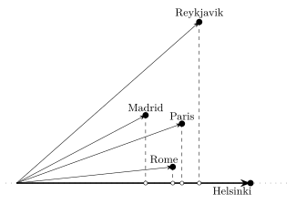
P-citiesFig. 2 illustrates inner products
between feature vectors in $\reals^{2}$ that represent
five European cities. Each city is characterized by its latitude
and longitude as its two features.
P-kernelMany ML methods access the feature vectors of data points only through inner products between feature vectors. A linear model uses hypotheses $\hypothesis(\featurevec) = \innerprod{\weights}{\featurevec}$. Consider regularized empirical risk minimization (RERM) over a training set $\trainset = \big\{ \big(\featurevec^{(\sampleidx)}, \truelabel^{(\sampleidx)}\big) \big\}_{\sampleidx=1}^{\samplesize}$, with a penalty that increases strictly with $\norm{\weights}$. It returns model parameters that are a linear combination of the feature vectors in the training set, $\widehat{\weights} = \sum_{\sampleidx=1}^{\samplesize} \expcoeff_{\sampleidx} \featurevec^{(\sampleidx)}$. This is the representer theorem, and the support-vector expansion of the support vector machine (SVM) is a special case of it (Schölkopf and Smola, 2002). The prediction for a new data point then reads \[ \learnthypothesis(\featurevec) = \sum_{\sampleidx=1}^{\samplesize} \expcoeff_{\sampleidx} \innerprod{\featurevec^{(\sampleidx)}}{\featurevec} \text{,} \] so training and prediction touch the feature vectors only through the inner products $\innerprod{\featurevec^{(\sampleidx)}}{\featurevec^{(\sampleidx')}}$ within the training set and $\innerprod{\featurevec^{(\sampleidx)}}{\featurevec}$ between the training set and the new data point. This is exploited by kernel methods that use a kernel $\kernel(\featurevec, \featurevec')$ to compute inner products without ever forming feature vectors (Schölkopf and Smola, 2002) (see kernel method).
P-distMethods built on Euclidean distances access the feature vectors only through inner products as well, even when they are defined without reference to one. The squared Euclidean distance between two feature vectors is a sum of three inner products, $\normgeneric{\featurevec - \featurevec'}{2}^{2} = \innerprod{\featurevec}{\featurevec} - 2 \innerprod{\featurevec}{\featurevec'} + \innerprod{\featurevec'}{\featurevec'}$. A method that uses the feature vectors only through their Euclidean distances therefore also uses them only through inner products. $k$-nearest neighbors ($k$-NN) is one example: it ranks the data points in the training set by the distance of their feature vectors to the feature vector of the new data point (Hastie et al., 2009, Sect. 2.3.2). The same kernel substitution therefore reaches it: by the identity above, each Euclidean distance is computed from three kernel evaluations, and no feature vector is ever formed.
Synonyms: scalar product, dot product.
See also: field, norm, vector, Hilbert space, orthogonality condition, metric space, Euclidean space, Cauchy-Schwarz inequality, orthogonal projection, kernel, kernel method, neuron, attention, principal component analysis, $k$-nearest neighbors.
@misc{dictml_innerproduct,
  author = {Jung, Alexander},
  title = {inner product},
  howpublished = {Dictionary of Applied Machine Learning (course edition)},
  year = {2026},
  doi = {10.5281/zenodo.21569296},
  note = {ISBN 978-952-64-3013-3, CC BY 4.0, retrieved 2026-08-21},
  url = {https://dictionaryofml.org/terms/innerproduct.html}
}