support vector machine

Typeset PDF version — the authoritative form of this entry

The support vector machine (SVM) is a binary classification method that learns a linear classifier by regularized empirical risk minimization (RERM), combining the hinge loss with a squared-norm penalty term. For a linearly separable training set the solution is the maximum-margin separating hyperplane. This hyperplane is fully determined by the feature vectors closest to it, which are called support vectors. The kernel SVM is obtained by combining the basic SVM with a feature map derived from a kernel function.

Definition

The support vector machine (SVM) is a binary classification method for data points with feature space $\featurespace=\reals^{\nrfeatures}$. In its simplest form, the SVM learns a linear classifier with decision boundary \[\{ \featurevec \in \reals^{\nrfeatures} : \weights^{\top} \featurevec + b = 0 \}.\] The linear classifier is parameterized by a vector $\weights \in \reals^{\nrfeatures} \setminus \{\mathbf{0}\}$ and $b \in \reals$. The vector $\weights$ is the normal vector to the decision boundary and the offset $b$ shifts the decision boundary away from the origin. For a data point with feature vector $\featurevec$ and label $\truelabel \in \{-1, +1\}$, the SVM delivers the prediction $\predictedlabel = \operatorname{sign}(\weights^{\top} \featurevec + b)$. SVMs have been applied to text classification, such as categorizing documents by topic, and to handwriting recognition, where each digit image is classified from pixel-level features (Cristianini and Shawe-Taylor, 2000).

The SVM can be formulated as an instance of regularized empirical risk minimization (RERM) over a training set: the model parameters $(\widehat{\weights}, \widehat{b})$ of the linear classifier are obtained as \begin{equation} \label{eq:svm_rerm} (\widehat{\weights}, \widehat{b}) = \argmin_{\weights \in \reals^{\nrfeatures},\, b \in \reals} \underbrace{\frac{1}{\samplesize} \sum_{\sampleidx=1}^{\samplesize} \max\{0,\, 1 - \truelabel^{(\sampleidx)} (\weights^{\top} \featurevec^{(\sampleidx)} + b)\} + \regparam \normgeneric{\weights}{2}^{2}}_{\defeq f(\weights, b)}\text{.} \end{equation} The SVM objective function consists of the average hinge loss on the training set plus a penalty term $\regparam \normgeneric{\weights}{2}^{2}$ with regularization parameter $\regparam > 0$ (Hastie et al., 2009, Sect. 12.3.2, p. 426; Shalev-Shwartz and Ben-David, 2014, Sect. 15.2, Eq. (15.5)). The penalty term in $\eqref{eq:svm_rerm}$ is almost the same as in ridge regression, except that the model parameter $b$ is left unpenalized.

Like logistic regression and linear regression, the SVM learns the model parameters $(\weights, b)$ of a linear model. In contrast to logistic regression and linear regression, the SVM objective function $f(\weights, b)$ is non-smooth because of the hinge loss. However, since the SVM objective function is convex, the optimization problem $\eqref{eq:svm_rerm}$ can be solved by convex optimization methods. One such method is subgradient descent which is obtained from gradient descent (GD) by replacing the gradient of the objective function with a subgradient (Shor, 1985; Bertsekas, 2016; Boyd and Vandenberghe, 2004).

Starting from an initial choice $\weights^{(0)}, b^{(0)}$ of the model parameters, subgradient descent repeatedly applies the update \[ \big(\weights^{(\iteridx+1)}, b^{(\iteridx+1)}\big) = \big(\weights^{(\iteridx)}, b^{(\iteridx)}\big) - \lrate^{(\iteridx)} \vg^{(\iteridx)} \text{, for } \iteridx = 0,1,\ldots \text{,} \] with a step size $\lrate^{(\iteridx)} > 0$ and a subgradient $\vg^{(\iteridx)} \in \partial f\big(\weights^{(\iteridx)}, b^{(\iteridx)}\big)$ of the SVM objective function $\eqref{eq:svm_rerm}$. Inserting the SVM objective function $\eqref{eq:svm_rerm}$ into the generic update yields the explicit update \[ \begin{aligned} \weights^{(\iteridx+1)} &= \big(1 - 2 \lrate^{(\iteridx)} \regparam\big) \weights^{(\iteridx)} + \frac{\lrate^{(\iteridx)}}{\samplesize} \sum_{\sampleidx=1}^{\samplesize} \expcoeff^{(\iteridx)}_{\sampleidx} \truelabel^{(\sampleidx)} \featurevec^{(\sampleidx)} \text{,} \\ b^{(\iteridx+1)} &= b^{(\iteridx)} + \frac{\lrate^{(\iteridx)}}{\samplesize} \sum_{\sampleidx=1}^{\samplesize} \expcoeff^{(\iteridx)}_{\sampleidx} \truelabel^{(\sampleidx)} \text{,} \end{aligned} \] with expansion coefficients $\expcoeff^{(\iteridx)}_{\sampleidx} \in [0, 1]$, for $\sampleidx = 1, \ldots, \samplesize$. The coefficient $\expcoeff^{(\iteridx)}_{\sampleidx}$ is nonzero only for a data point that satisfies $\truelabel^{(\sampleidx)} \big( \big(\weights^{(\iteridx)}\big)^{\top} \featurevec^{(\sampleidx)} + b^{(\iteridx)} \big) \leq 1$, i.e., a data point on which the hinge loss is nonzero or non-differentiable at the current model parameters. Each iteration scales $\weights^{(\iteridx)}$ by the factor $1 - 2 \lrate^{(\iteridx)} \regparam$ (the effect of the penalty term) and adds corrections $\truelabel^{(\sampleidx)} \featurevec^{(\sampleidx)}$ only from these data points. In particular, for the initialization $\weights^{(0)} = \mathbf{0}$, every iterate $\weights^{(\iteridx)}$ is a weighted sum $\sum_{\sampleidx=1}^{\samplesize} \expcoeff_{\sampleidx} \truelabel^{(\sampleidx)} \featurevec^{(\sampleidx)}$ of the feature vectors in the training set. The solution $\widehat{\weights}$ of $\eqref{eq:svm_rerm}$ admits the same expansion, with coefficients that are nonzero only for the data points satisfying the same condition $\truelabel^{(\sampleidx)} \big( \widehat{\weights}^{\top} \featurevec^{(\sampleidx)} + \widehat{b} \big) \leq 1$ (see below). For a suitably diminishing step size, e.g., $\lrate^{(\iteridx)} = 1/(\iteridx+1)$, the iterates $\big(\weights^{(\iteridx)}, b^{(\iteridx)}\big)$ converge to a solution of $\eqref{eq:svm_rerm}$ (Shor, 1985).

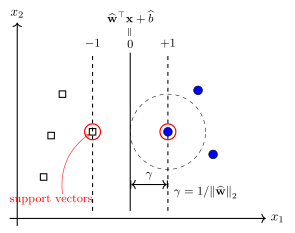
The solution of $\eqref{eq:svm_rerm}$ has a clear geometric meaning when the training set is linearly separable, i.e., there is some choice for $(\weights, b)$ such that $\operatorname{sign}(\weights^{\top} \featurevec^{(\sampleidx)} + b) \truelabel^{(\sampleidx)}=1$ for $\sampleidx=1, \ldots, \samplesize$. For a sufficiently small $\regparam$, the solution of $\eqref{eq:svm_rerm}$ determines the separating hyperplane that is farthest from the feature vectors in the training set (see Fig. 1). The distance between this hyperplane and the nearest feature vectors is referred to as the margin and is given by $1/\normgeneric{\widehat{\weights}}{2}$ (Boser et al., 1992; Cortes and Vapnik, 1995; Cristianini and Shawe-Taylor, 2000).

Figure 1 of the entry svm — Figure 1: Maximum-margin separation for a linearly separable training set. The decision boundary $\widehat{\weights}^{\top}\featurevec + \widehat{b} = 0$ (solid) lies halfway between two parallel hyperplanes $\widehat{\weights}^{\top}\featurevec + \widehat{b} = \pm 1$ (dashed). The support vectors (red) are the feature vectors that lie on these hyperplanes. The margin $\gamma = 1/\normgeneric{\widehat{\weights}}{2}$ is the distance from the decision boundary to the support vectors. Data points with label $\truelabel=+1$ are drawn as filled circles, those with $\truelabel=-1$ as open squares. The dashed circle of radius $\gamma$ shows that any support vector can be displaced by a perturbation with Euclidean norm less than $\gamma$ without crossing the decision boundary

The margin of the learned hyperplane measures robustness against perturbations of the features of a data point. Perturbing a feature vector $\featurevec$ by a vector $\boldsymbol{\delta}$ changes the score $\widehat{\weights}^{\top}\featurevec + \widehat{b}$ by $\widehat{\weights}^{\top}\boldsymbol{\delta}$, whose magnitude is at most $\normgeneric{\widehat{\weights}}{2} \normgeneric{\boldsymbol{\delta}}{2}$ by the Cauchy-Schwarz inequality. A data point therefore stays correctly classified under every feature perturbation with $\normgeneric{\boldsymbol{\delta}}{2} < \gamma$. Maximizing the margin maximizes this tolerated perturbation radius, so the maximum-margin classifier is the separating classifier that is robust against the largest feature perturbations (Xu et al., 2009).

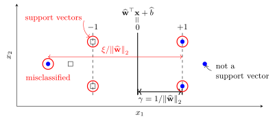
While the above discussion only applies when the SVM training set is linearly separable, every solution of the SVM problem $\eqref{eq:svm_rerm}$ has a structure that holds in general. In particular, \[\widehat{\weights} = \sum_{\sampleidx=1}^{\samplesize} \expcoeff_{\sampleidx} \truelabel^{(\sampleidx)} \featurevec^{(\sampleidx)}\] with expansion coefficients $\expcoeff_{\sampleidx} \geq 0$ that are nonzero only for the feature vectors with \[\truelabel^{(\sampleidx)} (\widehat{\weights}^{\top} \featurevec^{(\sampleidx)} + \widehat{b}) \leq 1.\] These feature vectors are referred to as support vectors since they entirely determine the SVM solution $(\widehat{\weights}, \widehat{b})$ (Boser et al., 1992; Cortes and Vapnik, 1995). Applying small perturbations to any feature vector which is not a support vector leaves $\widehat{\weights}$, $\widehat{b}$ unchanged (see Fig. 2).

Figure 2 of the entry svm — Figure 2: Non-separable toy training set in feature space $\reals^{2}$. The solution of the SVM problem $\eqref{eq:svm_rerm}$ places the decision boundary $\widehat{\weights}^{\top}\featurevec + \widehat{b} = 0$ between the two clusters, with margins $\widehat{\weights}^{\top}\featurevec + \widehat{b} = \pm 1$ at distance $\gamma = 1/\normgeneric{\widehat{\weights}}{2}$. The support vectors (red rings) are the four cluster points on the margins together with the outlier. The outlier, labeled $+1$, is misclassified beyond the opposite margin: $\truelabel(\widehat{\weights}^{\top}\featurevec + \widehat{b}) = -2 < -1$, with hinge loss value $\xi$. The two data points farther from the decision boundary than the margin are not support vectors. Data generated by `pythondemos/svm.py`

The basic SVM $\eqref{eq:svm_rerm}$ learns a linear classifier on the feature space $\featurespace = \reals^{\nrfeatures}$. It can be generalized to a classification method for data points whose feature vectors lie in an arbitrary feature space $\featurespace$ by first applying a feature map $\featuremap: \featurespace \to \featurespace'$ with $\featurespace' = \reals^{\nrfeatures}$, then learning a linear classifier on the transformed feature vectors. By choosing $\featuremap$ (and $\nrfeatures$) appropriately, any given training set can be made linearly separable in $\featurespace'$ (Cortes and Vapnik, 1995; Cristianini and Shawe-Taylor, 2000). A principled construction of a feature map $\featuremap$ is via a kernel $\kernel: \featurespace \times \featurespace \to \reals$. The resulting method is then referred to as a kernel SVM (Schölkopf and Smola, 2002).

Synonyms: maximum-margin classifier.

See also: binary classification, linear model, classifier, hinge loss, margin, hyperplane, decision boundary, robustness, ridge regression, least absolute shrinkage and selection operator, kernel, kernel method, subgradient descent.

References

Cristianini and Shawe-Taylor (2000). An Introduction to Support Vector Machines and Other Kernel-based Learning Methods. Cambridge Univ. Press.
Hastie et al. (2009). The Elements of Statistical Learning: Data Mining, Inference, and Prediction. Springer Science+Business Media.
Shalev-Shwartz and Ben-David (2014). Understanding Machine Learning: From Theory to Algorithms. Cambridge Univ. Press.
Shor (1985). Minimization Methods for Non-differentiable Functions. Springer.
Bertsekas (2016). Nonlinear Programming. Athena Scientific.
Boyd and Vandenberghe (2004). Convex Optimization. Cambridge Univ. Press.
Boser et al. (1992). A Training Algorithm for Optimal Margin Classifiers. Proc. 5th Annual Workshop on Computational Learning Theory (COLT).
Cortes and Vapnik (1995). Support-vector networks. Machine learning.
Xu et al. (2009). Robustness and Regularization of Support Vector Machines. J. Mach. Learn. Res..
Schölkopf and Smola (2002). Learning with Kernels: Support Vector Machines, Regularization, Optimization, and Beyond. MIT Press.

Cite this entry

@misc{dictml_svm,
  author = {Jung, Alexander},
  title = {support vector machine},
  howpublished = {Dictionary of Applied Machine Learning (course edition)},
  year = {2026},
  doi = {10.5281/zenodo.21569296},
  note = {ISBN 978-952-64-3013-3, CC BY 4.0, retrieved 2026-08-06},
  url = {https://dictionaryofml.org/terms/svm.html}
}