Dictionary of Applied Machine Learning
Typeset PDF version — the authoritative form of this entry
Python demo — a script that recomputes what this entry states and prints one line per check
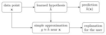
Explainable artificial intelligence (XAI) is the subfield of artificial intelligence (AI) concerned with making the predictions of machine learning (ML) methods understandable to humans. Much of it can be posed as a function approximation problem: a learned hypothesis is explained by a simpler function that a human can comprehend. Explanations differ in what they are made of. One kind reports a score for each feature, read off a linear map fitted near the data point (local interpretable model-agnostic explanations (LIME)) or obtained as additive contributions (SHapley Additive exPlanations (SHAP)). A counterfactual instead names another feature vector, the closest one whose prediction differs. A concept activation vector (CAV) states the explanation in a concept the user names, located in the activations inside the trained method. All three are post hoc and treat the learned hypothesis as fixed. The alternative is a hypothesis that needs no separate explanation, reached by restricting the hypothesis space to hypotheses a human comprehends or by regularization that favors explainable ones (explainable empirical risk minimization (EERM)).
Explainable artificial intelligence (XAI) is the subfield of artificial intelligence (AI) concerned with making the predictions of machine learning (ML) methods understandable to humans. It aims to complement each prediction by an explanation of how it has been obtained. If the ML method uses a sufficiently simple hypothesis space, the learned hypothesis may be inherently interpretable and no separate explanation is needed (Rudin, 2019); see interpretable machine learning (interpretable ML).
The term XAI was popularized by a program of the US Defense Advanced Research Projects Agency (Gunning and Aha, 2019); in the context of ML, the synonymous term explainable machine learning (explainable ML) is also used. The underlying property is explainability, which the international terminology standard for AI defines for artificial intelligence systems (AI systems) in general (Standardization and Commission, 2022, Sect. 3.5.7).
B-shapXAI can be posed as a function approximation problem. A trained
hypothesis
$\learnthypothesis: \featurespace \rightarrow \labelspace$,
e.g., delivered by an opaque deep net, is typically a
highly nonlinear function on a potentially
high-dimensional feature space $\featurespace$
(Goodfellow et al., 2016, Ch. 6). Explaining
$\learnthypothesis$ at a data point with feature vector
$\featurevec \in \featurespace$ means answering one question about
that function in a form a human can comprehend. The
examples of explanations below are of three kinds, distinguished
by what the explanation is made of. The first is a score for each
feature of the data point. The scores are read off a
simpler hypothesis out of a user-parseable hypothesis space that
agrees with $\learnthypothesis$ near $\featurevec$, for instance a
linear map whose weights are those scores, as fitted by
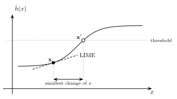
local interpretable model-agnostic explanations (LIME). Fig. 1 draws that
construction. The second is another
feature vector, one whose prediction differs. The third is a
concept the user names, located inside the trained method rather than
among the features of the data point. All three are post
hoc: they treat the learned hypothesis as fixed and construct
the explanation after training.
The third kind of explanation refers not to the features of the data point but to a concept the user specifies. Such a concept is defined by a dataset of examples the user supplies. A concept activation vector (CAV) locates such a concept as a direction in the space of the activations of one hidden layer of an artificial neural network (ANN): the normal vector of a decision boundary that separates the supplied examples carrying the concept from those that do not (Kim et al., 2018).
In contrast to LIME and counterfactual explanations, a CAV needs access to the internal computations of a machine learning system (ML system). One such internal computation is the activation $\vz = f(\featurevec)$ of a hidden layer in a deep net. A deep net computes $\learnthypothesis$ by feeding the activations $\vz$ to the final layers, which deliver a score $s(\vz)$ for each label; the prediction $\learnthypothesis(\featurevec)$ follows from those scores (see CAV). In an image classifier, for example, a user who suspects that photographs are labeled zebra through the concept "stripes" supplies photographs showing stripes and photographs not showing them. Each of these photographs results in an activation $\vz$ in the layer of interest. These activations are then used to fit a linear classifier that separates the two sets, and its normal vector is the CAV for "stripes". How much the concept contributed to the prediction of a zebra photograph is then measured by the directional derivative of the score $s$ along that CAV.
The above XAI methods construct an explanation after training, for a learned hypothesis that is already fixed. The alternative is to arrive at one that needs no separate explanation. Interpretable ML does so by admitting only hypotheses a human comprehends directly. This can be achieved by manually choosing a hypothesis space that is simple enough, or by regularization that favors hypotheses with specific properties, such as sparsity or predictability (Tibshirani, 1996; Zhang et al., 2024). Explainable empirical risk minimization (EERM) takes the second route for explainability: the user supplies their own predictions for the data points of a training set, and the penalty term charges the part of the learned hypothesis that those predictions do not already account for (Zhang et al., 2024).
Three aspects of an explanation are studied: whom it serves, how much of the learned hypothesis it covers, and whether it is faithful. How much an explanation achieves depends on who receives it: explainability is measured relative to a specific user (Colin et al., 2022; Jung and Nardelli, 2020). Explanations can be local, concerning a single prediction, or global, characterizing the learned hypothesis as a whole (Molnar, 2025).
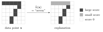
B-morfAn explanation must be faithful, i.e., reflect the computation that the learned hypothesis actually carries out. When the explanation scores the features, this can be tested rather than asserted. A CAM is faithful for a prediction if flipping the pixels it scores highest changes that prediction more often than flipping as many of the pixels it scores low. Perturbing the highest-scoring regions first and recording how quickly the predicted class score falls is the standard form of the test (Samek et al., 2017, Sect. III-C).
For the image of Fig. 2 and a linear classifier fitted to images of that kind, flipping the three highest-scoring pixels changes the prediction, while flipping the pixels in the opposite order leaves it unchanged through all $36$ of them; the map-guided order also changes the prediction sooner on each of $200$ noisy variants of the image. Faithfulness also limits what a post hoc explanation can achieve: one that agreed with the learned hypothesis everywhere would be that hypothesis itself, so a simpler explanation deviates from it somewhere (Rudin, 2019).
Two legal instruments explicitly state requirements on XAI. Under the general data protection regulation (GDPR), a person subjected to a decision taken by automated means is entitled to meaningful information about the logic involved in that decision (Parliament and Union, 2016, Art. 15(1)(h)). Communicating the algorithm itself is not a sufficiently concise and intelligible explanation (Union, 2025). Counterfactual information can be appropriate: the extent to which a variation in the personal data would have led to a different result. The second instrument is the EU AI Act, which requires for a high-risk artificial intelligence system (high-risk AI system) that affected persons obtain clear and meaningful explanations of the role of the AI system in the decision procedure (Parliament and Union, 2024, Art. 86) (see right to explanation).
Synonyms: explainable machine learning, explainable ML.
See also: explainability, interpretability, explanation, interpretable machine learning, explainable empirical risk minimization, local interpretable model-agnostic explanations, SHapley Additive exPlanations, counterfactual, feature, mechanistic interpretability, class activation map, right to explanation.
@misc{dictml_xaiterm,
  author = {Jung, Alexander},
  title = {explainable artificial intelligence},
  howpublished = {Dictionary of Applied Machine Learning (course edition)},
  year = {2026},
  doi = {10.5281/zenodo.21569296},
  note = {ISBN 978-952-64-3013-3, CC BY 4.0, retrieved 2026-08-21},
  url = {https://dictionaryofml.org/terms/xaiterm.html}
}