Dictionary of Applied Machine Learning
Typeset PDF version — the authoritative form of this entry
Python demo — a script that recomputes what this entry states and prints one line per check
An explanation accompanies a prediction delivered by a machine learning (ML) method and says what about the data point drove it. It can be text, a score per feature, a simple hypothesis that approximates the learned one near the data point, or a heat map over the regions of an image. Two requirements pull against each other: an explanation must be faithful, reflecting the computation the learned hypothesis carries out, and effective, letting the user it is written for anticipate the predictions it accompanies. An explanation that agreed with the learned hypothesis everywhere would be that hypothesis again, so a simpler one gives up faithfulness somewhere.
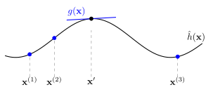
B-trainOne approach to enhance the transparency of a machine learning (ML) method for its human user is to provide an explanation alongside the predictions delivered by the method. Explanations can take different forms. For instance, they may consist of human-readable text or quantitative indicators, such as feature importance scores for the individual features of a given data point (Molnar, 2025). Fig.\ 1 illustrates two types of explanations. The first is a local linear approximation $g(\featurevec)$ of a nonlinear learned hypothesis $\learnthypothesis(\featurevec)$ around a specific feature vector $\featurevec'$, as used in the method local interpretable model-agnostic explanations (LIME). The second form of explanation depicted in the figure is a sparse set of predictions $\learnthypothesis(\featurevec^{(1)}), \learnthypothesis(\featurevec^{(2)}), \learnthypothesis(\featurevec^{(3)})$ at selected feature vectors, offering concrete reference points for the user. For a differentiable $\learnthypothesis$, the local linear approximation is the one determined by the gradient $\nabla \learnthypothesis(\featurevec')$, and the reference points are values of the same function.
A widely used form of explanation is a heat map: an intensity
map that scores each region of an image by how much it drove
the prediction, drawn over the image itself
(Selvaraju et al., 2017). For a convolutional neural network (CNN), those scores are read off
the network's own activations, which is what a
class activation map (CAM) does.
Faithful means that the explanation reflects the computation the learned hypothesis actually carries out, rather than one that is easier to present. A map over the pixels of an image is faithful when manipulating a few of the pixels it highlights changes the prediction while changing as many dark ones does not (see explainable artificial intelligence (XAI)). The two requirements are separate, and neither follows from the other. An unfaithful explanation can still be understandable and still let the user anticipate well, whenever it tracks the prediction without carrying anything about the computation: maps have been found that are independent of both the model parameters and the training set, yet look like the ones that are not (Adebayo et al., 2018). Such an explanation predicts by correlation, so it fails when the correlation does, and it cannot support a user who acts on the features it highlights.
The two requirements also pull against each other. An explanation that agreed with the learned hypothesis everywhere would be that hypothesis again, so a simpler explanation gives up faithfulness somewhere; where the hypothesis is itself simple enough to follow, it serves as its own explanation and none has to be constructed (see interpretable machine learning (interpretable ML)).
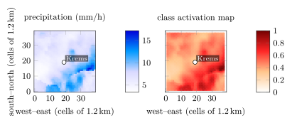
B-faithfulFig. 2 shows both requirements at
work on a prediction made from weather radar. The features are
the hourly precipitation over a 48 km box around Krems an der
Donau, and the prediction answers whether it will rain at
Krems two hours later. A CNN fitted to these images is
explained by a CAM, which scores each cell of
the image by how much it contributed to the prediction
(Selvaraju et al., 2017). For the hour drawn, the network is certain
of rain, and the map puts its weight on the band of precipitation
south-east of the town rather than on the rain already overhead.
Setting the precipitation to zero in the 160 cells the map scores
highest moves the predicted score by 3.32, against 0.64 for the 160
it scores lowest, and the map-guided cells move it further on 58 of
the 72 held-out hours.
pythondemos/explanation.py
@misc{dictml_explanation,
  author = {Jung, Alexander},
  title = {explanation},
  howpublished = {Dictionary of Applied Machine Learning (course edition)},
  year = {2026},
  doi = {10.5281/zenodo.21569296},
  note = {ISBN 978-952-64-3013-3, CC BY 4.0, retrieved 2026-08-19},
  url = {https://dictionaryofml.org/terms/explanation.html}
}