P-equiv writes when the script runsDictionary of Applied Machine Learning · regularization
Numerical companion to the entry regularization: it recomputes what the entry states and prints one line per check
One block per paragraph of the entry (marked [P...]): each block verifies numerically what the corresponding statement asserts. Self-contained (numpy/matplotlib only), fixed seed.
Run it with python3 regularization.py, from any directory — it writes its output files into the current directory. Requires NumPy and Matplotlib only, and uses fixed seeds, so the printed numbers reproduce exactly. Download regularization.py
One cell per block of the script: the code, and what that code printed when it last ran here
"""
regularization.py — numerical companion to the glossary entry
'regularization'.

One block per paragraph of the entry (marked [P...]): each block verifies
numerically what the corresponding statement asserts. Self-contained
(numpy/matplotlib only), fixed seed.

Blocks
------
[P-overfit] Plain ERM with a large model overfits: a degree-12
            polynomial on m = 15 points has near-zero training error
            and a large error on unseen data points.
[P-routes]  The three routes to regularization, each improving the
            error on unseen data points of the overfitting baseline:
            1) model pruning — shrink the hypothesis space (here: fit
               a smaller-degree polynomial, i.e., constrain higher
               coefficients to zero);
            2) loss penalization — add a penalty term (ridge);
            3) data augmentation — enlarge the trainset with perturbed
               copies of its data points.
[P-equiv]   The routes can coincide: data augmentation with zero-mean
            iid feature perturbations of variance sigma^2 yields
            (asymptotically in the number of perturbed copies) the same
            learned hypothesis as ridge regression with penalty
            sigma^2 ||w||^2 — verified by comparing the two learned
            parameter vectors.

Outputs
-------
regularization.png : preview figure (checking only).

Data generated by pythondemos/regularization.py.
"""

import numpy as np
import matplotlib

matplotlib.use("Agg")
import matplotlib.pyplot as plt

rng = np.random.default_rng(42)
report = []


def check(name, ok):
    report.append((name, bool(ok)))
    print(f"  [{'ok' if ok else 'FAIL'}] {name}")
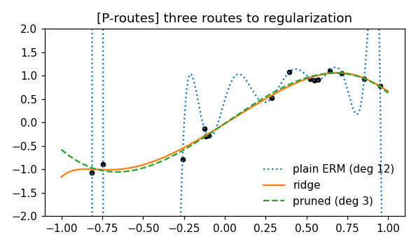
Plain ERM with a large model overfits: a degree-12 polynomial on m = 15 points has near-zero training error and a large error on unseen data points.
print("[P-overfit] plain ERM with a large model overfits")
m = 15
xtr = np.sort(rng.uniform(-1, 1, m))
ytr = np.sin(2.5 * xtr) + 0.2 * rng.normal(size=m)
xva = rng.uniform(-1, 1, 2000)
yva = np.sin(2.5 * xva) + 0.2 * rng.normal(size=2000)
deg = 12
V = np.vander(xtr, deg + 1)
Vva = np.vander(xva, deg + 1)
w_erm = np.linalg.lstsq(V, ytr, rcond=None)[0]
tr_erm = np.mean((ytr - V @ w_erm) ** 2)
va_erm = np.mean((yva - Vva @ w_erm) ** 2)
print(f"    ERM: train {tr_erm:.4f}, validation {va_erm:.2f}")
check("training error near zero", tr_erm < 0.01)
check("error on unseen data points far larger (overfitting)", va_erm > 10 * 0.04)
[P-overfit] plain ERM with a large model overfits
    ERM: train 0.0003, validation 11393397.53
  [ok] training error near zero
  [ok] error on unseen data points far larger (overfitting)
The three routes to regularization, each improving the error on unseen data points of the overfitting baseline: 1) model pruning — shrink the hypothesis space (here: fit a smaller-degree polynomial, i.e., constrain higher coefficients to zero); 2) loss penalization — add a penalty term (ridge); 3) data augmentation — enlarge the trainset with perturbed copies of its data points.
print("[P-routes] three routes, all improving validation error")
# 1) model pruning: shrink the hypothesis space H to degree-3 polynomials
c3 = np.polyfit(xtr, ytr, 3)
va_prune = np.mean((yva - np.polyval(c3, xva)) ** 2)
# 2) loss penalization: ridge on the degree-12 model
lam = 1e-3
w_ridge = np.linalg.solve(V.T @ V / m + lam * np.eye(deg + 1),
                          V.T @ ytr / m)
va_ridge = np.mean((yva - Vva @ w_ridge) ** 2)
# 3) data augmentation: perturbed copies of the data points
reps = 100
sigma = 0.1
x_aug = np.concatenate([xtr + sigma * rng.normal(size=m)
                        for _ in range(reps)])
y_aug = np.tile(ytr, reps)
w_aug = np.linalg.lstsq(np.vander(x_aug, deg + 1), y_aug, rcond=None)[0]
va_aug = np.mean((yva - Vva @ w_aug) ** 2)
print(f"    validation: ERM {va_erm:.2f} | prune {va_prune:.3f} | "
      f"ridge {va_ridge:.3f} | augment {va_aug:.3f}")
check("1) model pruning improves the error on unseen data points", va_prune < va_erm / 3)
check("2) loss penalization improves the error on unseen data points",
      va_ridge < va_erm / 3)
check("3) data augmentation improves the error on unseen data points",
      va_aug < va_erm / 3)
[P-routes] three routes, all improving validation error
    validation: ERM 11393397.53 | prune 0.042 | ridge 0.051 | augment 0.051
  [ok] 1) model pruning improves the error on unseen data points
  [ok] 2) loss penalization improves the error on unseen data points
  [ok] 3) data augmentation improves the error on unseen data points
The routes can coincide: data augmentation with zero-mean iid feature perturbations of variance sigma^2 yields (asymptotically in the number of perturbed copies) the same learned hypothesis as ridge regression with penalty sigma^2 ||w||^2 — verified by comparing the two learned parameter vectors.
print("[P-equiv] augmentation with sigma^2-noise = ridge with sigma^2")
# linear regression, feature perturbations with covariance sigma^2 I
mm, dd = 60, 3
X = rng.normal(size=(mm, dd))
y = X @ np.array([1.0, -0.5, 0.25]) + 0.1 * rng.normal(size=mm)
sig = 0.4
reps = 4000
Xa = np.vstack([X + sig * rng.normal(size=X.shape) for _ in range(reps)])
ya = np.tile(y, reps)
w_aug2 = np.linalg.lstsq(Xa, ya, rcond=None)[0]
w_ridge2 = np.linalg.solve(X.T @ X + mm * 0 + sig**2 * mm * np.eye(dd)
                           / 1, X.T @ y)  # (X^T X + m sig^2 I)^{-1} X^T y
diff = np.linalg.norm(w_aug2 - w_ridge2)
print(f"    ||w_augment - w_ridge|| = {diff:.4f}")
check("the augmented-ERM solution matches the ridge solution",
      diff < 0.02)

# ------------------------------------------------------------ preview
fig, ax = plt.subplots(figsize=(5.4, 3.2))
xx = np.linspace(-1, 1, 300)
ax.plot(xtr, ytr, "ko", ms=4)
ax.plot(xx, np.polyval(w_erm, xx), ":", label="plain ERM (deg 12)")
ax.plot(xx, np.polyval(w_ridge, xx), "-", label="ridge")
ax.plot(xx, np.polyval(c3, xx), "--", label="pruned (deg 3)")
ax.set_ylim(-2, 2); ax.legend(frameon=False)
ax.set_title("[P-routes] three routes to regularization")
fig.tight_layout()
fig.savefig("regularization.png", dpi=110)
print(f"\n{sum(ok for _, ok in report)}/{len(report)} checks passed")
assert all(ok for _, ok in report)
[P-equiv] augmentation with sigma^2-noise = ridge with sigma^2
    ||w_augment - w_ridge|| = 0.0019
  [ok] the augmented-ERM solution matches the ridge solution

6/6 checks passed
P-equiv writes when the script runs