P-specify writes when the script runsDictionary of Applied Machine Learning · probability distribution
Numerical companion to the entry probability distribution: it recomputes what the entry states and prints one line per check
One block per paragraph of the entry (marked [P...]): each block verifies numerically what the corresponding statement asserts. Self-contained (numpy/matplotlib only), fixed seed.
Run it with python3 probdist.py, from any directory — it writes its output files into the current directory. Requires NumPy and Matplotlib only, and uses fixed seeds, so the printed numbers reproduce exactly. Download probdist.py
One cell per block of the script: the code, and what that code printed when it last ran here
"""
probdist.py — numerical companion to the glossary entry
'probability distribution'.

One block per paragraph of the entry (marked [P...]): each block verifies
numerically what the corresponding statement asserts. Self-contained
(numpy/matplotlib only), fixed seed.

The method used throughout is the simplest one available: it reads a data
set of numbers and returns their average, which is the hypothesis that
minimizes the average squared error loss over all constant hypotheses. That
keeps every quantity below available in closed form, so a check compares a
measured number against a formula rather than against another simulation.

Blocks
------
[P-method]  One distribution, many data sets, a different output each time:
            the outputs of the method have a spread of their own, and that
            spread shrinks as sigma/sqrt(m) with the data set size m.
[P-typical] The distribution decides which data points are typical (relative
            frequencies of a growing sample converge to it), and the two
            numbers attached to the method — the training error on the data
            set it was given, and the risk on a fresh data point — are random
            as well. Their gap shrinks like 2*sigma^2/m, which is what
            generalization asserts here; the check is against the Monte
            Carlo error of the estimate, not a hand-picked tolerance.
[P-specify] How a distribution is specified: a binary RV by the single
            probability P(y = 0), and a continuous real-valued RV by a pdf p,
            for which P(x in [a, b]) ~ p(a)|b - a| on a short interval.

Outputs
-------
probdist.png : preview figure (checking only).

Data generated by pythondemos/probdist.py.
"""

import numpy as np
import matplotlib

matplotlib.use("Agg")
import matplotlib.pyplot as plt

rng = np.random.default_rng(42)
report = []

MU, SIGMA = 1.0, 2.0            # the common distribution: N(MU, SIGMA^2)
NR_DATASETS = 4000


def check(name, ok):
    report.append((name, bool(ok)))
    print(f"  [{'ok' if ok else 'FAIL'}] {name}")


def method(data):
    """The ML method: the average, i.e. the constant hypothesis minimizing
    the average squared error loss on `data`."""
    return float(np.mean(data))
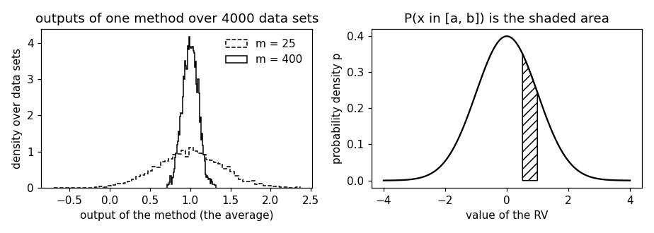
One distribution, many data sets, a different output each time: the outputs of the method have a spread of their own, and that spread shrinks as sigma/sqrt(m) with the data set size m.
print("[P-method] one distribution, many data sets, a different output each time")
outputs = {}
for m in (25, 400):
    outputs[m] = np.array([method(rng.normal(MU, SIGMA, m))
                           for _ in range(NR_DATASETS)])
spread = {m: float(np.std(out)) for m, out in outputs.items()}
print(f"    output spread: {spread[25]:.4f} at m=25, {spread[400]:.4f} at m=400"
      f"  (sigma/sqrt(m) = {SIGMA / np.sqrt(25):.4f}, "
      f"{SIGMA / np.sqrt(400):.4f})")
check("two data sets from the same distribution give different outputs",
      outputs[25][0] != outputs[25][1])
check("the spread of the outputs shrinks with the data set size",
      spread[400] < spread[25])
for m in (25, 400):
    check(f"the spread matches sigma/sqrt(m) within 5% at m={m}",
          abs(spread[m] - SIGMA / np.sqrt(m)) / (SIGMA / np.sqrt(m)) < 0.05)
[P-method] one distribution, many data sets, a different output each time
    output spread: 0.4034 at m=25, 0.0979 at m=400  (sigma/sqrt(m) = 0.4000, 0.1000)
  [ok] two data sets from the same distribution give different outputs
  [ok] the spread of the outputs shrinks with the data set size
  [ok] the spread matches sigma/sqrt(m) within 5% at m=25
  [ok] the spread matches sigma/sqrt(m) within 5% at m=400
The distribution decides which data points are typical (relative frequencies of a growing sample converge to it), and the two numbers attached to the method — the training error on the data set it was given, and the risk on a fresh data point — are random as well. Their gap shrinks like 2*sigma^2/m, which is what generalization asserts here; the check is against the Monte Carlo error of the estimate, not a hand-picked tolerance.
print("[P-typical] typical data points, and the two random numbers of the method")
p_true = np.array([0.5, 0.3, 0.2])              # distribution on {0, 1, 2}
errs = []
for m in (10**2, 10**4, 10**6):
    draws = rng.choice(3, size=m, p=p_true)
    errs.append(np.max(np.abs(np.bincount(draws, minlength=3) / m - p_true)))
print(f"    max |frequency - p| for m=1e2,1e4,1e6: "
      f"{errs[0]:.4f}, {errs[1]:.4f}, {errs[2]:.4f}")
check("relative frequencies converge to the distribution", errs[0] > errs[2])
check("frequencies at m=1e6 within 2e-3 of the distribution", errs[2] < 2e-3)

# For the average as hypothesis, both numbers are available in closed form:
# the training error is the sample variance, and the risk on a fresh data
# point is SIGMA^2 + (output - MU)^2. Their expected gap is 2*SIGMA^2/m.
gaps = {}
for m in (25, 400):
    data = rng.normal(MU, SIGMA, (NR_DATASETS, m))
    out = data.mean(axis=1)
    trainerr = ((data - out[:, None]) ** 2).mean(axis=1)
    risk = SIGMA ** 2 + (out - MU) ** 2
    gaps[m] = float(np.mean(risk - trainerr))
    # the gap is itself averaged over data sets, so it carries a Monte Carlo
    # error; comparing against the formula only makes sense relative to that
    stderr = float(np.std(risk - trainerr) / np.sqrt(NR_DATASETS))
    print(f"    m={m:>3}: training error {trainerr.mean():.4f}, "
          f"risk {risk.mean():.4f}, gap {gaps[m]:.4f} +- {stderr:.4f} "
          f"(2*sigma^2/m = {2 * SIGMA ** 2 / m:.4f})")
    check(f"the gap agrees with 2*sigma^2/m at m={m} "
          f"(within three standard errors)",
          abs(gaps[m] - 2 * SIGMA ** 2 / m) < 3 * stderr)
check("training error and risk move closer as m grows", gaps[400] < gaps[25])
[P-typical] typical data points, and the two random numbers of the method
    max |frequency - p| for m=1e2,1e4,1e6: 0.1200, 0.0010, 0.0004
  [ok] relative frequencies converge to the distribution
  [ok] frequencies at m=1e6 within 2e-3 of the distribution
    m= 25: training error 3.8156, risk 4.1630, gap 0.3474 +- 0.0179 (2*sigma^2/m = 0.3200)
  [ok] the gap agrees with 2*sigma^2/m at m=25 (within three standard errors)
    m=400: training error 3.9861, risk 4.0104, gap 0.0243 +- 0.0046 (2*sigma^2/m = 0.0200)
  [ok] the gap agrees with 2*sigma^2/m at m=400 (within three standard errors)
  [ok] training error and risk move closer as m grows
How a distribution is specified: a binary RV by the single probability P(y = 0), and a continuous real-valued RV by a pdf p, for which P(x in [a, b]) ~ p(a)|b - a| on a short interval.
print("[P-specify] one probability specifies a binary RV; a pdf a continuous one")
p0 = 0.73
y = (rng.uniform(size=10**6) >= p0).astype(int)   # P(y = 0) = p0
f0 = float(np.mean(y == 0))
check("empirical P(y = 0) recovers p0 = 0.73", abs(f0 - p0) < 2e-3)
check("P(y = 1) = 1 - P(y = 0)", np.isclose(np.mean(y == 1), 1 - f0))

pdf = lambda t: np.exp(-t ** 2 / 2) / np.sqrt(2 * np.pi)
x = rng.standard_normal(10**7)
a = 0.5
rel_errs = []
for width in (0.5, 0.1, 0.02):
    p_emp = np.mean((x >= a) & (x <= a + width))
    rel_errs.append(abs(p_emp - pdf(a) * width) / p_emp)
print(f"    relative approximation error for |b-a|=0.5,0.1,0.02: "
      f"{rel_errs[0]:.3f}, {rel_errs[1]:.3f}, {rel_errs[2]:.3f}")
check("the pdf approximation improves as the interval shrinks",
      rel_errs[0] > rel_errs[1] > rel_errs[2])
check("relative error below 1% for |b - a| = 0.02", rel_errs[2] < 0.01)

# ------------------------------------------------------------ preview
fig, ax = plt.subplots(1, 2, figsize=(8.4, 3.0))
for m, style in ((25, "--"), (400, "-")):
    ax[0].hist(outputs[m], bins=60, histtype="step", density=True,
               color="k", linestyle=style, label=f"m = {m}")
ax[0].set_xlabel("output of the method (the average)")
ax[0].set_ylabel("density over data sets")
ax[0].set_title("outputs of one method over 4000 data sets")
ax[0].legend(frameon=False)

t = np.linspace(-4, 4, 400)
ax[1].plot(t, pdf(t), "k-")
ax[1].fill_between(t, pdf(t), where=(t >= a) & (t <= a + 0.5),
                   facecolor="none", hatch="///", edgecolor="k")
ax[1].set_xlabel("value of the RV")
ax[1].set_ylabel("probability density p")
ax[1].set_title("P(x in [a, b]) is the shaded area")
fig.tight_layout()
fig.savefig("probdist.png", dpi=110)

print(f"\n{sum(ok for _, ok in report)}/{len(report)} checks passed")
assert all(ok for _, ok in report)
[P-specify] one probability specifies a binary RV; a pdf a continuous one
  [ok] empirical P(y = 0) recovers p0 = 0.73
  [ok] P(y = 1) = 1 - P(y = 0)
    relative approximation error for |b-a|=0.5,0.1,0.02: 0.175, 0.028, 0.006
  [ok] the pdf approximation improves as the interval shrinks
  [ok] relative error below 1% for |b - a| = 0.02

13/13 checks passed
P-specify writes when the script runs