B-backprop writes when the script runsDictionary of Applied Machine Learning · gradient
Numerical companion to the entry gradient: it recomputes what the entry states and prints one line per check
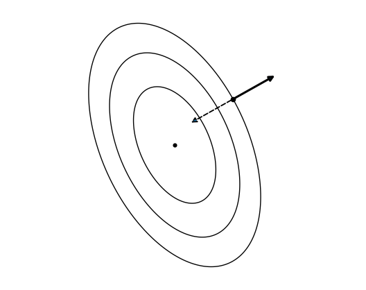
Verifies, for the quadratic f(w) = (1/2) w^T Q w with Q = [[2, 0.6], [0.6, 1]], the defining and geometric properties of the gradient stated in the entry, and generates the level-set data for the entry's figure. Self-contained (numpy/matplotlib only), deterministic.
Run it with python3 pythondemos/gradient.py, from the repository root — it writes its data files under pythondemos/. Requires NumPy and Matplotlib only, and uses fixed seeds, so the printed numbers reproduce exactly. Download gradient.py
One cell per block of the script: the code, and what that code printed when it last ran here
"""
gradient.py — numerical companion to the glossary entry 'gradient'.

Purpose
-------
Verifies, for the quadratic f(w) = (1/2) w^T Q w with
Q = [[2, 0.6], [0.6, 1]], the defining and geometric properties of the
gradient stated in the entry, and generates the level-set data for the
entry's figure.  Self-contained (numpy/matplotlib only), deterministic.

Blocks
------
[B-fd]       The analytic gradient grad f(w') = Q w' matches central finite
             differences at w' = (1.4, 1.1) to 1e-8.
[B-taylor]   Local linear approximation: the error
             |f(w) - f(w') - grad^T (w - w')| / ||w - w'|| vanishes as
             w -> w' (ratio decreases by ~10x per 10x step shrink).
[B-steepest] Among 720 unit directions d, the directional derivative
             grad^T d is maximized by d = grad/||grad|| (within 0.5 deg).
[B-orth]     The directional derivative along the level-set tangent at w'
             is zero (up to 1e-12): the gradient is orthogonal to the
             level set.
[B-partials] Partial derivatives alone do not guarantee a gradient for a
             non-convex function: g(w) = w1 w2^2 / (w1^2 + w2^4) has both
             partials equal to 0 at the origin, yet the linear-
             approximation error ratio DIVERGES along w = (t^2, t) — no
             gradient exists there (the entry's convexity assumption is
             not dispensable).
[B-hilbert]  Inner-product dependence of the gradient: w.r.t. the inner
             product <u,v>_M = u^T M v (an SPD M), the gradient of f at
             w' is M^{-1} Q w'. It represents the directional derivative
             (<M^{-1} Q w', d>_M = (Q w')^T d for all d) and is the
             steepest-ascent direction among 720 directions of unit
             M-norm.
[B-min]      At the minimizer w-hat = 0 of f, the gradient vanishes.
[B-erm]      ML relevance: for a synthetic training set (m = 30) and a
             linear regression, the analytic ERM
             gradient -(2/m) sum (y - w^T x) x matches finite
             differences, vanishes at the least-squares solution, and
             one GD step decreases the objective.
[B-backprop] For a one-hidden-layer network with tanh activation, the
             gradient of the ERM objective computed by backpropagation
             (chain rule, layer by layer) matches finite differences on
             all weights.

Outputs
-------
gradient_levelsets.csv : polylines of three level sets f(w) = const.
                         through and inside w' (columns x,y; nan rows
                         separate the level sets) for the entry's pgfplots
                         figure.
gradient.png           : matplotlib preview of the figure (checking only).

The figure's gradient arrow at w' is the unit vector of
grad f(w') = Q w' = (3.46, 1.94); its coordinates are printed below and
used verbatim in the entry's TikZ code.
"""

import numpy as np                  # the only numerical dependency
import matplotlib                   # imported before pyplot to set the backend

matplotlib.use("Agg")               # non-interactive backend: no display needed
import matplotlib.pyplot as plt    # plotting API for the preview figure

report = []                         # collects (check name, pass/fail) pairs


def check(name, ok):                # records and prints one verification
    report.append((name, bool(ok)))               # store the verdict
    print(f"  [{'ok' if ok else 'FAIL'}] {name}")  # echo it immediately


Q = np.array([[2.0, 0.6], [0.6, 1.0]])  # SPD matrix defining f(w) = w^T Q w / 2


def f(w):                           # the quadratic objective f(w) = (1/2) w^T Q w
    # einsum contracts w_i Q_ij w_j over the LAST axis, so w may be a
    # single point (shape (2,)) or a whole grid (shape (..., 2))
    return 0.5 * np.einsum("...i,ij,...j->...", w, Q, w)


def grad(w):                        # analytic gradient of f: grad f(w) = Q w
    return Q @ w                    # matrix-vector product


wp = np.array([1.4, 1.1])           # the point w' marked in the entry's figure
g = grad(wp)                        # gradient at w' (drawn as the solid arrow)
The analytic gradient grad f(w') = Q w' matches central finite differences at w' = (1.4, 1.1) to 1e-8.
eps = 1e-6                          # half-width of the finite-difference stencil
# central difference (f(w'+eps e_j) - f(w'-eps e_j)) / (2 eps) per coordinate
g_fd = np.array([(f(wp + eps * e) - f(wp - eps * e)) / (2 * eps)
                 for e in np.eye(2)])
check("[B-fd]       analytic gradient matches finite differences",
      np.linalg.norm(g - g_fd) < 1e-8)           # entries agree to 1e-8
[ok] [B-fd] analytic gradient matches finite differences
Local linear approximation: the error |f(w) - f(w') - grad^T (w - w')| / ||w - w'|| vanishes as w -> w' (ratio decreases by ~10x per 10x step shrink).
rng = np.random.default_rng(0)      # fixed seed: deterministic direction
d = rng.standard_normal(2)          # a random approach direction
d /= np.linalg.norm(d)              # normalized so ||w - w'|| = h below
ratios = []                         # error ratios for shrinking displacements h
for h in (1e-1, 1e-2, 1e-3):        # three decades of displacement h
    w = wp + h * d                  # approach point w = w' + h d
    # the entry's defining ratio |f(w) - f(w') - g^T (w - w')| / ||w - w'||
    ratios.append(abs(f(w) - f(wp) - g @ (w - wp)) / h)
check("[B-taylor]   linear-approximation error ratio vanishes",
      # for a quadratic the ratio is O(h): each 10x shrink of h must shrink
      # the ratio ~10x (the 1.5 slack absorbs rounding)
      ratios[0] > 9 * ratios[1] > 81 * ratios[2] / 1.5)
[ok] [B-taylor] linear-approximation error ratio vanishes
Among 720 unit directions d, the directional derivative grad^T d is maximized by d = grad/||grad|| (within 0.5 deg).
angles = np.linspace(0.0, 2.0 * np.pi, 720, endpoint=False)  # 0.5-degree grid
dirs = np.c_[np.cos(angles), np.sin(angles)]  # 720 unit direction vectors
best = dirs[np.argmax(dirs @ g)]    # direction maximizing the directional derivative g^T d
# angle (in degrees) between that maximizer and the normalized gradient
ang_err = np.degrees(np.arccos(np.clip(best @ (g / np.linalg.norm(g)),
                                       -1.0, 1.0)))
check("[B-steepest] gradient direction maximizes directional derivative",
      ang_err < 0.5)                # agreement within the grid resolution
[ok] [B-steepest] gradient direction maximizes directional derivative
The directional derivative along the level-set tangent at w' is zero (up to 1e-12): the gradient is orthogonal to the level set.
t = np.array([-g[1], g[0]]) / np.linalg.norm(g)   # level-set tangent: rotate g by 90 deg
check("[B-orth]     zero directional derivative along the level set",
      abs(g @ t) < 1e-12)           # g^T t = 0: gradient orthogonal to the level set
[ok] [B-orth] zero directional derivative along the level set
Partial derivatives alone do not guarantee a gradient for a non-convex function: g(w) = w1 w2^2 / (w1^2 + w2^4) has both partials equal to 0 at the origin, yet the linear- approximation error ratio DIVERGES along w = (t^2, t) — no gradient exists there (the entry's convexity assumption is not dispensable).
# g(w) = w1 w2^2 / (w1^2 + w2^4): both partials exist (= 0) at the origin,
# but g is not differentiable there (g is not convex).
def g_cex(w1, w2):                  # the counterexample function
    den = w1 ** 2 + w2 ** 4         # denominator, zero only at the origin
    # define g(0,0) = 0 (its limit along both axes); elsewhere the formula
    return np.where(den == 0.0, 0.0, w1 * w2 ** 2 / den)


eps = 1e-6                          # finite-difference half-width (as in [B-fd])
px = (g_cex(eps, 0.0) - g_cex(-eps, 0.0)) / (2 * eps)  # partial w.r.t. w1 at 0
py = (g_cex(0.0, eps) - g_cex(0.0, -eps)) / (2 * eps)  # partial w.r.t. w2 at 0
# along w = (t^2, t), g = 1/2 while ||w|| -> 0: the error ratio
# |g(w) - 0 - 0| / ||w|| blows up, so no gradient exists at 0.
ratios_cex = [abs(g_cex(t ** 2, t)) / np.hypot(t ** 2, t)
              for t in (1e-1, 1e-2, 1e-3)]
check("[B-partials] partials exist at 0 but the error ratio diverges",
      # partials vanish exactly, and the ratio GROWS ~10x per decade
      abs(px) < 1e-12 and abs(py) < 1e-12
      and ratios_cex[2] > 9 * ratios_cex[1] > 81 * ratios_cex[0] / 1.5)
[ok] [B-partials] partials exist at 0 but the error ratio diverges
Inner-product dependence of the gradient: w.r.t. the inner product <u,v>_M = u^T M v (an SPD M), the gradient of f at w' is M^{-1} Q w'. It represents the directional derivative (<M^{-1} Q w', d>_M = (Q w')^T d for all d) and is the steepest-ascent direction among 720 directions of unit M-norm.
M = np.array([[2.0, 0.5], [0.5, 1.0]])            # SPD inner-product matrix
gM = np.linalg.solve(M, g)                        # gradient w.r.t. <.,.>_M: M^{-1} Q w'
rng_h = np.random.default_rng(1)    # fixed seed: deterministic test directions
D = rng_h.standard_normal((100, 2))  # 100 random directions d
check("[B-hilbert]  <g_M, d>_M equals the directional derivative g^T d",
      # representation property: d^T M g_M = d^T g for every d
      np.allclose(D @ M @ gM, D @ g, atol=1e-12))
# rescale the 720 directions from [B-steepest] to unit M-norm ||d||_M = 1
dirs_M = dirs / np.sqrt(np.einsum("ij,jk,ik->i", dirs, M, dirs))[:, None]
best_M = dirs_M[np.argmax(dirs_M @ g)]  # maximizer of the directional derivative g^T d
check("[B-hilbert]  steepest ascent w.r.t. the M-norm is along g_M",
      # angle between that maximizer and g_M is below the grid resolution
      np.degrees(np.arccos(np.clip(
          best_M @ gM / (np.linalg.norm(best_M) * np.linalg.norm(gM)),
          -1.0, 1.0))) < 0.5)
  [ok] [B-hilbert]  <g_M, d>_M equals the directional derivative g^T d
  [ok] [B-hilbert]  steepest ascent w.r.t. the M-norm is along g_M
At the minimizer w-hat = 0 of f, the gradient vanishes.
check("[B-min]      gradient vanishes at the minimizer w-hat = 0",
      np.linalg.norm(grad(np.zeros(2))) == 0.0)   # grad f(0) = Q 0 = 0 exactly
[ok] [B-min] gradient vanishes at the minimizer w-hat = 0
ML relevance: for a synthetic training set (m = 30) and a linear regression, the analytic ERM gradient -(2/m) sum (y - w^T x) x matches finite differences, vanishes at the least-squares solution, and one GD step decreases the objective.
# linear regression: f(w) = (1/m) sum (y - w^T x)^2 with
# gradient -(2/m) sum (y - w^T x) x, as displayed in the entry.
rng_e = np.random.default_rng(2)    # fixed seed: reproducible training set
m = 30                              # size of the training set
X = rng_e.standard_normal((m, 2))   # rows are the feature vectors x^(r)
y = X @ np.array([1.0, -0.5]) + 0.1 * rng_e.standard_normal(m)  # noisy labels


def f_erm(w):                       # the ERM objective: average squared error
    return np.mean((y - X @ w) ** 2)


def grad_erm(w):                    # its analytic gradient: -(2/m) X^T (y - X w)
    return -(2.0 / m) * X.T @ (y - X @ w)


w0 = np.array([0.4, 0.8])           # an arbitrary (non-optimal) parameter vector
# central finite differences of f_erm at w0, coordinate by coordinate
g_erm_fd = np.array([(f_erm(w0 + eps * e) - f_erm(w0 - eps * e)) / (2 * eps)
                     for e in np.eye(2)])
check("[B-erm]      analytic ERM gradient matches finite differences",
      np.linalg.norm(grad_erm(w0) - g_erm_fd) < 1e-8)  # agree to 1e-8
w_hat = np.linalg.lstsq(X, y, rcond=None)[0]  # least-squares solution (ERM minimizer)
check("[B-erm]      ERM gradient vanishes at the least-squares solution",
      np.linalg.norm(grad_erm(w_hat)) < 1e-10)  # zero-gradient condition at w-hat
check("[B-erm]      one GD step decreases the ERM objective",
      f_erm(w0 - 0.1 * grad_erm(w0)) < f_erm(w0))  # step along -grad with lrate 0.1
  [ok] [B-erm]      analytic ERM gradient matches finite differences
  [ok] [B-erm]      ERM gradient vanishes at the least-squares solution
  [ok] [B-erm]      one GD step decreases the ERM objective
For a one-hidden-layer network with tanh activation, the gradient of the ERM objective computed by backpropagation (chain rule, layer by layer) matches finite differences on all weights.
# one-hidden-layer network h(x) = w2^T tanh(W1 x); the gradient of the ERM
# objective via the chain rule (backpropagation) vs finite differences.
rng_b = np.random.default_rng(3)    # fixed seed: reproducible weights
W1 = rng_b.standard_normal((3, 2)) * 0.5  # hidden-layer weights (3 units, 2 inputs)
w2 = rng_b.standard_normal(3) * 0.5       # output-layer weights


def f_net(W1_, w2_):                # ERM objective of the network on (X, y)
    return np.mean((y - np.tanh(X @ W1_.T) @ w2_) ** 2)


A = np.tanh(X @ W1.T)                              # m x 3 activations (forward pass)
res = y - A @ w2                                   # m residuals y - h(x)
dpred = -(2.0 / m) * res                           # dL/dprediction, per sample
gb_w2 = A.T @ dpred                                # backprop: output layer (dL/dw2)
# hidden layer: chain rule through tanh' = 1 - A^2, then through W1 x
gb_W1 = ((dpred[:, None] * (1.0 - A ** 2) * w2).T @ X)   # hidden layer
theta_fd = []                       # finite-difference gradient, same parameter order
for i in range(3):                  # loop over hidden units ...
    for j in range(2):              # ... and input coordinates
        P = np.zeros_like(W1); P[i, j] = eps  # perturbation of one W1 entry
        # central difference w.r.t. that single entry
        theta_fd.append((f_net(W1 + P, w2) - f_net(W1 - P, w2)) / (2 * eps))
for i in range(3):                  # loop over the output-layer weights
    p = np.zeros(3); p[i] = eps     # perturbation of one w2 entry
    theta_fd.append((f_net(W1, w2 + p) - f_net(W1, w2 - p)) / (2 * eps))
check("[B-backprop] backprop gradient matches finite differences",
      # flatten (W1, w2) backprop gradients and compare to the stencil
      np.linalg.norm(np.r_[gb_W1.ravel(), gb_w2] - theta_fd) < 1e-8)

# --------------------------------------------------------------- level sets
G = 500                             # grid resolution per axis
# the grid must contain the outermost level set f(w) = f(w') entirely
# (max |w_2| on it is sqrt(2 f(w') (Q^{-1})_{22}) ~ 2.92): a too-small grid
# clips the contour and the closing segment below draws a straight chord.
gx = np.linspace(-3.2, 3.6, G)      # horizontal grid coordinates
gy = np.linspace(-3.2, 3.2, G)      # vertical grid coordinates
GX, GY = np.meshgrid(gx, gy)        # full 2-D evaluation grid
F = f(np.stack([GX, GY], axis=-1))  # f evaluated on the whole grid at once
levels = [0.8, 2.0, float(f(wp))]   # two inner levels plus the level through w'

fig0, ax0 = plt.subplots()          # throwaway figure: only the contour data is used
cs = ax0.contour(GX, GY, F, levels=levels)  # compute the three contour polylines
plt.close(fig0)                     # discard the figure, keep the contour set

with open("pythondemos/gradient_levelsets.csv", "w") as fh:  # pgfplots data file
    fh.write("x,y\n")               # column header expected by \addplot table
    first = True                    # tracks whether a nan separator is needed
    for segs in cs.allsegs:         # one entry per contour level ...
        for s in segs:              # ... each holding its polyline segments
            if not first:           # between polylines ...
                fh.write("nan,nan\n")  # ... a nan row breaks the pgfplots path
            first = False           # subsequent polylines need the separator
            for p in s[::5]:        # every 5th vertex suffices at print size
                fh.write(f"{p[0]:.4f},{p[1]:.4f}\n")  # one vertex per row
            if np.allclose(s[0], s[-1]):          # close closed loops only
                fh.write(f"{s[0][0]:.4f},{s[0][1]:.4f}\n")  # repeat first vertex

u = g / np.linalg.norm(g) * 1.2     # unit gradient arrow, scaled to length 1.2
# print the arrow coordinates that the entry's TikZ code uses verbatim
print(f"\nw' = {wp} | grad f(w') = {g} | unit arrow (len 1.2) = "
      f"({u[0]:.2f}, {u[1]:.2f})")

# -------------------------------------------------------------- preview
fig, ax = plt.subplots(figsize=(4.8, 3.8))  # preview canvas (checking only)
ax.contour(GX, GY, F, levels=levels, colors="k", linewidths=0.9)  # level sets
ax.plot(*wp, "ko", ms=4)            # mark the point w'
ax.annotate("", xy=wp + u, xytext=wp,   # solid arrow: the gradient at w'
            arrowprops=dict(arrowstyle="-|>", lw=2))
ax.annotate("", xy=wp - u, xytext=wp,   # dashed arrow: the negative gradient
            arrowprops=dict(arrowstyle="-|>", lw=1.2, linestyle="--"))
ax.plot(0, 0, "k.", ms=6)           # mark the minimizer w-hat = 0
ax.set_aspect("equal")              # equal axis scaling (as in the TikZ figure)
ax.set_axis_off()                   # the entry's figure has no axes either
fig.tight_layout()                  # trim whitespace
fig.savefig("pythondemos/gradient.png", dpi=110)  # write the preview PDF

n_ok = sum(ok for _, ok in report)  # count the passed checks
print(f"{n_ok}/{len(report)} checks pass")  # summary line
print("wrote pythondemos/gradient_levelsets.csv, pythondemos/gradient.png")
if n_ok != len(report):             # any failed check ...
    raise SystemExit(1)             # ... makes the script exit non-zero
  [ok] [B-backprop] backprop gradient matches finite differences

w' = [1.4 1.1] | grad f(w') = [3.46 1.94] | unit arrow (len 1.2) = (1.05, 0.59)
12/12 checks pass
wrote pythondemos/gradient_levelsets.csv, pythondemos/gradient.png
B-backprop writes when the script runs