P-maxent writes when the script runsDictionary of Applied Machine Learning · Gaussian random variable
Numerical companion to the entry Gaussian random variable: it recomputes what the entry states and prints one line per check
One block per paragraph of the entry (marked [P...]): each block verifies numerically what the corresponding statement asserts. Self-contained (numpy/matplotlib only), fixed seed.
Run it with python3 gaussrv.py, from any directory — it writes its output files into the current directory. Requires NumPy and Matplotlib only, and uses fixed seeds, so the printed numbers reproduce exactly. Download gaussrv.py
One cell per block of the script: the code, and what that code printed when it last ran here
"""
gaussrv.py — numerical companion to the glossary entry
'Gaussian random variable (Gaussian RV)'.

One block per paragraph of the entry (marked [P...]): each block verifies
numerically what the corresponding statement asserts. Self-contained
(numpy/matplotlib only), fixed seed.

Blocks
------
[P-std]     The standard Gaussian pdf integrates to one, and draws have
            mean ~ 0 and variance ~ 1; the general Gaussian RV
            x' = sigma x + mu has mean mu and variance sigma^2.
[P-vector]  The construction x = A z + mu with iid standard Gaussian z
            yields a Gaussian random vector with mean mu and covariance
            A A^T = C (checked empirically).
[P-process] A Gaussian random vector restricted to a subset of its
            entries is again Gaussian with the corresponding sub-mean
            and sub-covariance (the finite-restriction property behind
            Gaussian processes; checked via mean/covariance of the
            restriction).
[P-clt]     Central limit theorem: standardized averages of iid uniform
            (non-Gaussian) RVs approach the standard Gaussian — the
            empirical cdf distance to the Gaussian cdf shrinks as the
            number of averaged RVs grows.
[P-maxent]  Maximum-uncertainty property: among distributions with the
            same variance, the Gaussian has the largest differential
            entropy — its analytic entropy exceeds the (analytic)
            entropies of the uniform and Laplace distributions matched
            to variance one.

Outputs
-------
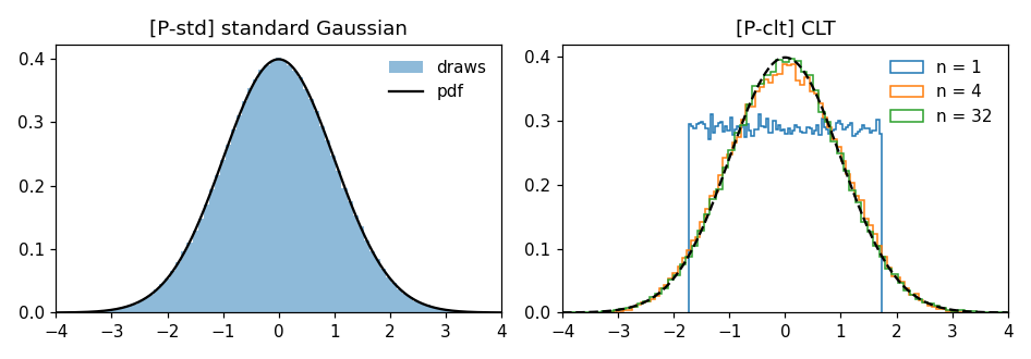
gaussrv.png : preview figure (checking only).

Data generated by pythondemos/gaussrv.py.
"""

import numpy as np
import matplotlib

matplotlib.use("Agg")
import matplotlib.pyplot as plt

rng = np.random.default_rng(42)
report = []


def check(name, ok):
    report.append((name, bool(ok)))
    print(f"  [{'ok' if ok else 'FAIL'}] {name}")
The standard Gaussian pdf integrates to one, and draws have mean ~ 0 and variance ~ 1; the general Gaussian RV x' = sigma x + mu has mean mu and variance sigma^2.
print("[P-std] standard and general scalar Gaussian RV")
pdf = lambda t: np.exp(-t**2 / 2) / np.sqrt(2 * np.pi)
t = np.linspace(-8, 8, 20001)
check("pdf integrates to one", abs(np.trapezoid(pdf(t), t) - 1) < 1e-9)
z = rng.standard_normal(10**6)
check("draws: mean ~ 0, variance ~ 1",
      abs(z.mean()) < 3e-3 and abs(z.var() - 1) < 3e-3)
mu_s, sigma_s = -1.5, 2.0
xp = sigma_s * z + mu_s
check("sigma z + mu has mean mu and variance sigma^2",
      abs(xp.mean() - mu_s) < 6e-3 and abs(xp.var() - sigma_s**2) < 2e-2)
[P-std] standard and general scalar Gaussian RV
  [ok] pdf integrates to one
  [ok] draws: mean ~ 0, variance ~ 1
  [ok] sigma z + mu has mean mu and variance sigma^2
The construction x = A z + mu with iid standard Gaussian z yields a Gaussian random vector with mean mu and covariance A A^T = C (checked empirically).
print("[P-vector] x = A z + mu has mean mu, covariance A A^T")
A = np.array([[1.0, 0.0, 0.0], [0.5, 0.8, 0.0], [-0.2, 0.3, 1.1]])
mu = np.array([1.0, 2.0, -1.0])
C = A @ A.T
Z = rng.standard_normal((10**6, 3))
Xv = Z @ A.T + mu
check("empirical mean matches mu",
      np.max(np.abs(Xv.mean(axis=0) - mu)) < 6e-3)
check("empirical covariance matches C = A A^T",
      np.max(np.abs(np.cov(Xv.T, ddof=0) - C)) < 8e-3)
[P-vector] x = A z + mu has mean mu, covariance A A^T
  [ok] empirical mean matches mu
  [ok] empirical covariance matches C = A A^T
A Gaussian random vector restricted to a subset of its entries is again Gaussian with the corresponding sub-mean and sub-covariance (the finite-restriction property behind Gaussian processes; checked via mean/covariance of the restriction).
print("[P-process] restrictions of a Gaussian vector stay Gaussian")
sub = [0, 2]
check("restricted mean is the sub-vector of mu",
      np.max(np.abs(Xv[:, sub].mean(axis=0) - mu[sub])) < 6e-3)
check("restricted covariance is the sub-matrix of C",
      np.max(np.abs(np.cov(Xv[:, sub].T, ddof=0)
                    - C[np.ix_(sub, sub)])) < 8e-3)
[P-process] restrictions of a Gaussian vector stay Gaussian
  [ok] restricted mean is the sub-vector of mu
  [ok] restricted covariance is the sub-matrix of C
Central limit theorem: standardized averages of iid uniform (non-Gaussian) RVs approach the standard Gaussian — the empirical cdf distance to the Gaussian cdf shrinks as the number of averaged RVs grows.
print("[P-clt] averages of iid uniform RVs approach the Gaussian")
from math import erf
Phi = np.vectorize(lambda s: 0.5 * (1 + erf(s / np.sqrt(2))))
grid = np.linspace(-3, 3, 121)
dists = []
for n in [1, 4, 32]:
    u = rng.uniform(-0.5, 0.5, size=(10**5, n))
    s = u.mean(axis=1) * np.sqrt(12 * n)        # standardized average
    ecdf = (s[:, None] <= grid[None, :]).mean(axis=0)
    dists.append(np.max(np.abs(ecdf - Phi(grid))))
print(f"    sup |ecdf - Phi| for n=1,4,32: "
      f"{dists[0]:.3f}, {dists[1]:.3f}, {dists[2]:.3f}")
check("cdf distance to the Gaussian shrinks as n grows",
      dists[0] > dists[1] > dists[2])
check("n = 32 average is Gaussian to within 0.01", dists[2] < 0.01)
[P-clt] averages of iid uniform RVs approach the Gaussian
    sup |ecdf - Phi| for n=1,4,32: 0.058, 0.008, 0.002
  [ok] cdf distance to the Gaussian shrinks as n grows
  [ok] n = 32 average is Gaussian to within 0.01
Maximum-uncertainty property: among distributions with the same variance, the Gaussian has the largest differential entropy — its analytic entropy exceeds the (analytic) entropies of the uniform and Laplace distributions matched to variance one.
print("[P-maxent] Gaussian maximizes entropy at fixed variance")
h_gauss = 0.5 * np.log(2 * np.pi * np.e)          # variance 1
h_unif = 0.5 * np.log(12)                          # uniform, variance 1
h_lap = 1 + 0.5 * np.log(2 * 1 / 2)                # Laplace b=1/sqrt(2)
check("h(Gauss) > h(uniform) at variance one", h_gauss > h_unif)
check("h(Gauss) > h(Laplace) at variance one", h_gauss > h_lap)

# ------------------------------------------------------------ preview
fig, ax = plt.subplots(1, 2, figsize=(8.6, 3.0))
ax[0].hist(z, bins=100, density=True, alpha=0.5, label="draws")
ax[0].plot(t, pdf(t), "k-", label="pdf")
ax[0].set_xlim(-4, 4); ax[0].legend(frameon=False)
ax[0].set_title("[P-std] standard Gaussian")
for n, c in zip([1, 4, 32], ("C0", "C1", "C2")):
    u = rng.uniform(-0.5, 0.5, size=(10**5, n))
    ax[1].hist(u.mean(axis=1) * np.sqrt(12 * n), bins=80, density=True,
               histtype="step", color=c, label=f"n = {n}")
ax[1].plot(t, pdf(t), "k--"); ax[1].set_xlim(-4, 4)
ax[1].legend(frameon=False); ax[1].set_title("[P-clt] CLT")
fig.tight_layout()
fig.savefig("gaussrv.png", dpi=110)
print(f"\n{sum(ok for _, ok in report)}/{len(report)} checks passed")
assert all(ok for _, ok in report)
[P-maxent] Gaussian maximizes entropy at fixed variance
  [ok] h(Gauss) > h(uniform) at variance one
  [ok] h(Gauss) > h(Laplace) at variance one

11/11 checks passed
P-maxent writes when the script runs