P-fixedpoint writes when the script runsDictionary of Applied Machine Learning · empirical risk minimization
Numerical companion to the entry empirical risk minimization: it recomputes what the entry states and prints one line per check
One block per paragraph of the entry (marked [P...]): each block verifies numerically what the corresponding statement asserts. Self-contained (numpy/matplotlib only), fixed seed.
Run it with python3 erm.py, from any directory — it writes its output files into the current directory. Requires NumPy and Matplotlib only, and uses fixed seeds, so the printed numbers reproduce exactly. Download erm.py
One cell per block of the script: the code, and what that code printed when it last ran here
"""
erm.py — numerical companion to the glossary entry
'empirical risk minimization (ERM)'.

One block per paragraph of the entry (marked [P...]): each block verifies
numerically what the corresponding statement asserts. Self-contained
(numpy/matplotlib only), fixed seed.

Blocks
------
[P-risk]       The risk of a hypothesis is the expected loss under the
               data-generating distribution; the ideal choice minimizes
               the risk (verified on a grid of hypotheses against a
               large Monte Carlo sample).
[P-surrogate]  The distribution is unknown; ERM minimizes the
               sample-average surrogate. As the trainset grows, the
               risk of the ERM hypothesis approaches the minimal risk
               (consistency of the surrogate).
[P-map]        ERM is a map A: trainset -> learned hypothesis. For
               the linear model with squared error loss the map has a closed
               form, its output attains the minimal empirical risk, and
               calling it on different trainsets yields different
               learned hypotheses.
[P-fixedpoint] In practice A is computed by an iterative optimization
               method that is a fixed-point iteration: the GD update
               operator T has the ERM solution as its fixed point
               (T(w-hat) = w-hat), and iterating T converges to it.

Outputs
-------
erm.png : preview figure (checking only).

Data generated by pythondemos/erm.py.
"""

import numpy as np
import matplotlib

matplotlib.use("Agg")
import matplotlib.pyplot as plt

rng = np.random.default_rng(42)
report = []


def check(name, ok):
    report.append((name, bool(ok)))
    print(f"  [{'ok' if ok else 'FAIL'}] {name}")


# data-generating distribution: y = 2 x + 1 + noise, x ~ U(0, 10)
W_TRUE = np.array([2.0, 1.0])
def draw(m):
    x = rng.uniform(0, 10, m)
    y = W_TRUE[0] * x + W_TRUE[1] + 0.5 * rng.normal(size=m)
    return x, y

def risk(w, mc=200000):                            # expected squared loss
    x, y = draw(mc)
    return np.mean((y - w[0] * x - w[1]) ** 2)
The risk of a hypothesis is the expected loss under the data-generating distribution; the ideal choice minimizes the risk (verified on a grid of hypotheses against a large Monte Carlo sample).
print("[P-risk] risk = expected loss; the ideal hypothesis minimizes it")
cands = [np.array([a, b]) for a in (1.5, 2.0, 2.5) for b in (0.0, 1.0)]
risks = [risk(w) for w in cands]
best = cands[int(np.argmin(risks))]
check("the risk-minimizing candidate is the true hypothesis (2, 1)",
      np.array_equal(best, W_TRUE))
check("its risk equals the noise floor 0.25 (irreducible)",
      abs(min(risks) - 0.25) < 0.01)
[P-risk] risk = expected loss; the ideal hypothesis minimizes it
  [ok] the risk-minimizing candidate is the true hypothesis (2, 1)
  [ok] its risk equals the noise floor 0.25 (irreducible)
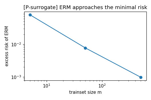
The distribution is unknown; ERM minimizes the sample-average surrogate. As the trainset grows, the risk of the ERM hypothesis approaches the minimal risk (consistency of the surrogate).
print("[P-surrogate] ERM minimizes the sample-average surrogate")
def erm_fit(m):
    x, y = draw(m)
    return np.polyfit(x, y, 1)
excess = [np.mean([risk(erm_fit(m)) - 0.25 for _ in range(20)])
          for m in (5, 50, 500)]
print(f"    excess risk of ERM at m = 5, 50, 500: "
      f"{excess[0]:.4f}, {excess[1]:.4f}, {excess[2]:.5f}")
check("the ERM hypothesis approaches the minimal risk as m grows",
      excess[0] > excess[1] > excess[2] > 0)
[P-surrogate] ERM minimizes the sample-average surrogate
    excess risk of ERM at m = 5, 50, 500: 0.0791, 0.0077, 0.00099
  [ok] the ERM hypothesis approaches the minimal risk as m grows
ERM is a map A: trainset -> learned hypothesis. For the linear model with squared error loss the map has a closed form, its output attains the minimal empirical risk, and calling it on different trainsets yields different learned hypotheses.
print("[P-map] ERM is a map from trainsets to hypotheses")
x1, y1 = draw(30)
x2, y2 = draw(30)
A = lambda x, y: np.polyfit(x, y, 1)
w1, w2 = A(x1, y1), A(x2, y2)
emp = lambda w, x, y: np.mean((y - w[0] * x - w[1]) ** 2)
check("A(D) attains the minimal empirical risk on D (vs perturbations)",
      all(emp(w1 + d, x1, y1) > emp(w1, x1, y1)
          for d in ([0.05, 0], [-0.05, 0], [0, 0.2], [0, -0.2])))
check("different trainsets yield different learned hypotheses",
      not np.allclose(w1, w2))
[P-map] ERM is a map from trainsets to hypotheses
  [ok] A(D) attains the minimal empirical risk on D (vs perturbations)
  [ok] different trainsets yield different learned hypotheses
In practice A is computed by an iterative optimization method that is a fixed-point iteration: the GD update operator T has the ERM solution as its fixed point (T(w-hat) = w-hat), and iterating T converges to it.
print("[P-fixedpoint] the optimizer is a fixed-point iteration")
X = np.c_[x1, np.ones(30)]
w_hat = np.linalg.solve(X.T @ X, X.T @ y1)         # ERM solution
L = 2 * np.linalg.eigvalsh(X.T @ X / 30).max()
T = lambda w: w - (1 / L) * (2 / 30) * X.T @ (X @ w - y1)   # GD operator
check("the ERM solution is a fixed point: T(w-hat) = w-hat",
      np.allclose(T(w_hat), w_hat, atol=1e-10))
w = np.zeros(2)
for _ in range(60000):     # ill-conditioned (x vs intercept): slow rate
    w = T(w)
check("iterating T converges to the ERM solution",
      np.linalg.norm(w - w_hat) < 1e-5)

# ------------------------------------------------------------ preview
fig, ax = plt.subplots(figsize=(4.8, 3.2))
ax.loglog([5, 50, 500], excess, "o-")
ax.set_xlabel("trainset size m"); ax.set_ylabel("excess risk of ERM")
ax.set_title("[P-surrogate] ERM approaches the minimal risk")
fig.tight_layout()
fig.savefig("erm.png", dpi=110)
print(f"\n{sum(ok for _, ok in report)}/{len(report)} checks passed")
assert all(ok for _, ok in report)
[P-fixedpoint] the optimizer is a fixed-point iteration
  [ok] the ERM solution is a fixed point: T(w-hat) = w-hat
  [ok] iterating T converges to the ERM solution

7/7 checks passed
P-fixedpoint writes when the script runs