B-fig writes when the script runsDictionary of Applied Machine Learning · concept activation vector
Numerical companion to the entry concept activation vector: it recomputes what the entry states and prints one line per check
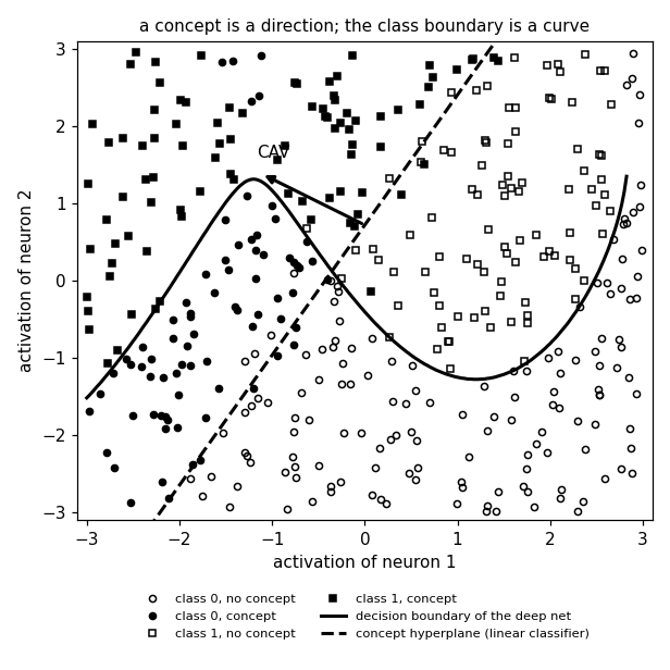
A CAV is fitted the way the entry describes it, in a plane a reader can look at: the activations of two neurons of one hidden layer. A deep net separates two classes in that plane by a decision boundary that is far from a straight line, while the concept ("stripes") is separated from the non-concept examples by a hyperplane whose normal vector is the CAV. The two boundaries are different objects, and drawing them in the same plane is what the entry's figure does.
Run it with python3 pythondemos/cav.py, from the repository root — it writes its data files under pythondemos/. Requires NumPy and Matplotlib only, and uses fixed seeds, so the printed numbers reproduce exactly. Download cav.py
One cell per block of the script: the code, and what that code printed when it last ran here
"""
cav.py — numerical companion to the glossary entry 'concept activation
vector (CAV)'.

Purpose
-------
A CAV is fitted the way the entry describes it, in a plane a reader can
look at: the activations of two neurons of one hidden layer.  A deep net
separates two classes in that plane by a decision boundary that is far
from a straight line, while the concept ("stripes") is separated from the
non-concept examples by a hyperplane whose normal vector is the CAV.  The
two boundaries are different objects, and drawing them in the same plane
is what the entry's figure does.

The activations are synthetic, since a real network's layer has hundreds
of neurons and no two of them span a plane worth drawing.  Everything
computed from them is real: the linear classifier is fitted to the
supplied examples, the CAV is its weight vector, and the conceptual sensitivity is
the directional derivative of the network's score along that vector.

Self-contained (numpy + matplotlib only), fixed seed.

Blocks
------
[B-plane]  The plane of activations: two classes whose boundary curves,
           and a concept that occupies a half-plane.  A linear classifier
           fitted to the CLASS labels does poorly, which is what makes
           the network's boundary nonlinear rather than a line in
           disguise.
[B-cav]    The CAV: a binary linear classifier separating concept from
           non-concept activations, fitted to the supplied examples.
           It
           reaches high accuracy, and its weight vector -- the CAV -- is
           the normal of the separating hyperplane.
[B-tcav]   Conceptual sensitivity: the directional derivative of the
           network's score along the unit CAV, averaged over the data
           points of one class.  The concept the network uses raises the
           score at about two thirds of them -- 73% is the ceiling for
           any direction here, since a curved boundary bends away from
           every straight line -- while
           the concept planted orthogonal to it sits at chance.  Random directions are reported for context
           and are NOT the discriminator: where the score varies in one
           direction across the plane, a whole cone of directions scores as well as the
           right one, so the comparison that carries information is
           between the two concepts.
[B-fig]    The figure: scatter of both classes, the network's curved
           boundary, the CAV hyperplane, and the CAV itself.  Written to
           cav_points.csv, cav_boundary.csv, cav_cavline.csv and cav.png.

Outputs
-------
cav_points.csv   : z1, z2, class, concept for every activation vector
cav_boundary.csv : the network's decision boundary in the plane
cav_cavline.csv  : the concept hyperplane and the CAV arrow
cav.png          : preview (checking only)
"""

import numpy as np
import matplotlib

matplotlib.use("Agg")
import matplotlib.pyplot as plt

report = []                         # collects (check name, pass/fail) pairs


def check(name, ok):                # records and prints one verification
    report.append((name, bool(ok)))
    print(f"  [{'ok' if ok else 'FAIL'}] {name}")


rng = np.random.default_rng(20260819)
M = 400                             # activation vectors drawn
400 activation vectors, 182 in class 1, 164 carrying the concept
The plane of activations: two classes whose boundary curves, and a concept that occupies a half-plane. A linear classifier fitted to the CLASS labels does poorly, which is what makes the network's boundary nonlinear rather than a line in disguise.
# The plane is spanned by the activations of two neurons of one hidden layer.
Z = rng.uniform(-3.0, 3.0, size=(M, 2))
z1, z2 = Z[:, 0], Z[:, 1]

# The network's score in this plane. Its zero set is the decision boundary
# drawn in the entry's figure: a curve, not a line.
def net_score(a, b):
    return 1.6 * np.sin(1.15 * a) + 0.9 * b - 0.35 * a - 0.25 * b ** 2 + 0.4


cls = (net_score(z1, z2) > 0).astype(int)          # the network's two classes

# A concept occupies a half-plane: it is a DIRECTION in activation space,
# which is the assumption a CAV rests on. Two concepts are planted. The first
# lies along the direction the network's score actually varies in, averaged
# over the points of class 1; the second lies orthogonal to it, and the
# network's score barely moves along it. A test that could not tell these
# apart would say nothing.
slope = np.stack([1.6 * 1.15 * np.cos(1.15 * z1) - 0.35, 0.9 - 0.5 * z2], 1)
g = slope[net_score(z1, z2) > 0].mean(axis=0)
w_used = g / np.linalg.norm(g)                     # the direction the net uses
w_idle = np.array([-w_used[1], w_used[0]])         # orthogonal to it
concept = ((Z @ w_used + rng.normal(0, 0.28, M)) > 0.35).astype(int)
concept_idle = ((Z @ w_idle + rng.normal(0, 0.28, M)) > 0.35).astype(int)

print(f"  {M} activation vectors, {cls.sum()} in class 1, "
      f"{concept.sum()} carrying the concept")
check("[B-plane] both classes and both concept sets are populated",
      80 < cls.sum() < M - 80 and 80 < concept.sum() < M - 80)


def fit_linear(X, y, steps=4000, lrate=0.35):
    """Logistic regression by gradient descent; returns (weights, bias)."""
    w, b = np.zeros(X.shape[1]), 0.0
    for _ in range(steps):
        p = 1.0 / (1.0 + np.exp(-(X @ w + b)))
        w -= lrate * X.T @ (p - y) / len(y)
        b -= lrate * (p - y).mean()
    return w, b


acc = lambda w, b, X, y: float((((X @ w + b) > 0) == (y > 0.5)).mean())

w_cls, b_cls = fit_linear(Z, cls.astype(float))
print(f"  a straight line fitted to the CLASS labels reaches accuracy "
      f"{acc(w_cls, b_cls, Z, cls):.2f}")
check("[B-plane] the network's boundary is not a line in disguise",
      acc(w_cls, b_cls, Z, cls) < 0.85)
  [ok] [B-plane] both classes and both concept sets are populated
  a straight line fitted to the CLASS labels reaches accuracy 0.82
  [ok] [B-plane] the network's boundary is not a line in disguise
  concept classifier accuracy 0.95; the CAV points along (-0.86, 0.51), cos to the planted direction 0.999
The CAV: a binary linear classifier separating concept from non-concept activations, fitted to the supplied examples. It reaches high accuracy, and its weight vector -- the CAV -- is the normal of the separating hyperplane.
w_cav, b_cav = fit_linear(Z, concept.astype(float))
cav = w_cav / np.linalg.norm(w_cav)                # the CAV, unit length
acc_cav = acc(w_cav, b_cav, Z, concept)
cos = float(cav @ w_used)
print(f"  concept classifier accuracy {acc_cav:.2f}; the CAV points along "
      f"({cav[0]:.2f}, {cav[1]:.2f}), cos to the planted direction {cos:.3f}")
check("[B-cav] concept and non-concept activations are linearly separable",
      acc_cav > 0.92)
check("[B-cav] the CAV recovers the direction the concept was planted along",
      cos > 0.98)
w_cav_idle, b_cav_idle = fit_linear(Z, concept_idle.astype(float))
cav_idle = w_cav_idle / np.linalg.norm(w_cav_idle)
  [ok] [B-cav] concept and non-concept activations are linearly separable
  [ok] [B-cav] the CAV recovers the direction the concept was planted along
  moving along the CAV of the used concept raises the score at 65% of the class-1 points, along the CAV of the other concept at 52%; random directions 49% on average, and 18% of them do as well
Conceptual sensitivity: the directional derivative of the network's score along the unit CAV, averaged over the data points of one class. The concept the network uses raises the score at about two thirds of them -- 73% is the ceiling for any direction here, since a curved boundary bends away from every straight line -- while the concept planted orthogonal to it sits at chance. Random directions are reported for context and are NOT the discriminator: where the score varies in one direction across the plane, a whole cone of directions scores as well as the right one, so the comparison that carries information is between the two concepts.
# Conceptual sensitivity: the directional derivative of the network's score
# along the unit CAV, evaluated at the data points of class 1.
EPS = 1e-4


def directional_derivative(direction, points):
    d = direction / np.linalg.norm(direction)
    ahead = net_score(points[:, 0] + EPS * d[0], points[:, 1] + EPS * d[1])
    here = net_score(points[:, 0], points[:, 1])
    return (ahead - here) / EPS


pts = Z[cls == 1]
frac = lambda v: float((directional_derivative(v, pts) > 0).mean())
frac_used, frac_idle = frac(cav), frac(cav_idle)
rand_frac = np.array([frac(rng.normal(size=2)) for _ in range(200)])
print(f"  moving along the CAV of the used concept raises the score at "
      f"{frac_used:.0%} of the class-1 points, along the CAV of the other "
      f"concept at {frac_idle:.0%}; random directions {rand_frac.mean():.0%} "
      f"on average, and {(rand_frac >= frac_used).mean():.0%} of them do as "
      f"well")
# 73% is what the best direction reaches here: the boundary is curved, so
# the direction the score rises in turns across the plane and none raises it
# everywhere. A demo tuned until this number was near 1 would have a nearly
# straight boundary, which is not what a deep net's looks like.
check("[B-tcav] the used concept raises the score at most class-1 points",
      frac_used > 0.6)
check("[B-tcav] the concept the network does not use scores near chance",
      abs(frac_idle - 0.5) < 0.2)
  [ok] [B-tcav] the used concept raises the score at most class-1 points
  [ok] [B-tcav] the concept the network does not use scores near chance
  wrote pythondemos/cav_points.csv, cav_boundary.csv, cav_cavline.csv, cav_arrow.csv
  wrote pythondemos/cav.png

6/6 checks passed
The figure: scatter of both classes, the network's curved boundary, the CAV hyperplane, and the CAV itself. Written to cav_points.csv, cav_boundary.csv, cav_cavline.csv and cav.png.
with open("pythondemos/cav_points.csv", "w") as fh:
    # grp joins the two labels into one symbolic column, which is what
    # pgfplots' scatter/classes needs to give each kind its own marker
    fh.write("z1,z2,class,concept,grp\n")
    for (a, b), c, k in zip(Z, cls, concept):
        fh.write(f"{a:.4f},{b:.4f},{c},{k},c{c}k{k}\n")

# the network's boundary, traced as z2 for each z1 where the score vanishes
grid1 = np.linspace(-3, 3, 241)
with open("pythondemos/cav_boundary.csv", "w") as fh:
    fh.write("z1,z2\n")
    for a in grid1:
        bs = np.linspace(-3, 3, 2001)
        s = net_score(np.full_like(bs, a), bs)
        sign = np.where(np.diff(np.sign(s)))[0]
        if len(sign):
            fh.write(f"{a:.4f},{bs[sign[0]]:.4f}\n")

# the concept hyperplane w . z + b = 0, and the CAV drawn from a point on it
with open("pythondemos/cav_cavline.csv", "w") as fh:
    fh.write("z1,z2\n")
    for a in np.linspace(-3, 3, 61):
        fh.write(f"{a:.4f},{(-b_cav - w_cav[0] * a) / w_cav[1]:.4f}\n")
foot = np.array([0.0, -b_cav / w_cav[1]])
with open("pythondemos/cav_arrow.csv", "w") as fh:
    fh.write("z1,z2\n")
    fh.write(f"{foot[0]:.4f},{foot[1]:.4f}\n")
    fh.write(f"{foot[0] + 1.3 * cav[0]:.4f},{foot[1] + 1.3 * cav[1]:.4f}\n")
print("  wrote pythondemos/cav_points.csv, cav_boundary.csv, "
      "cav_cavline.csv, cav_arrow.csv")

fig, ax = plt.subplots(figsize=(5.6, 5.6))
for c, mark, lbl in ((0, "o", "class 0"), (1, "s", "class 1")):
    for k, fill in ((0, "none"), (1, "k")):
        sel = (cls == c) & (concept == k)
        ax.plot(Z[sel, 0], Z[sel, 1], mark, ms=4, mfc=fill, mec="k", lw=0,
                label=f"{lbl}, {'concept' if k else 'no concept'}")
bnd = np.loadtxt("pythondemos/cav_boundary.csv", delimiter=",", skiprows=1)
ax.plot(bnd[:, 0], bnd[:, 1], "k-", lw=2.0,
        label="decision boundary of the deep net")
line = np.loadtxt("pythondemos/cav_cavline.csv", delimiter=",", skiprows=1)
ax.plot(line[:, 0], line[:, 1], "k--", lw=2.0,
        label="concept hyperplane (linear classifier)")
ax.annotate("", xy=foot + 1.3 * cav, xytext=foot,
            arrowprops=dict(arrowstyle="-|>", lw=2.0, color="k"))
ax.annotate("CAV", foot + 1.5 * cav + np.array([0.12, 0.10]), fontsize=10)
ax.set_xlim(-3.1, 3.1)
ax.set_ylim(-3.1, 3.1)
ax.set_xlabel("activation of neuron 1")
ax.set_ylabel("activation of neuron 2")
ax.set_title("a concept is a direction; the class boundary is a curve",
             fontsize=10)
# below the axes: the plane is populated everywhere, so any in-axes
# placement covers data
ax.legend(frameon=False, fontsize=7.5, loc="upper center",
          bbox_to_anchor=(0.5, -0.13), ncol=2)
fig.tight_layout()
fig.savefig("pythondemos/cav.png", dpi=110)
print("  wrote pythondemos/cav.png")

bad = [n for n, ok in report if not ok]
print(f"\n{len(report) - len(bad)}/{len(report)} checks passed"
      + (f"; FAILED: {bad}" if bad else ""))
B-fig writes when the script runs